U-Net is the most widely used architecture in medical image segmentation. If you have worked in this space for more than a week, you have encountered it.
But most explanations of U-Net either go straight to diagrams without explaining why the architecture is shaped the way it is, or they go so deep into the mathematics that the core idea gets buried.
This post takes a different approach. Before showing you the architecture, it explains the problem that forced the architecture into existence. Once you understand the problem, the design makes complete sense, and you will remember it in a way that a diagram alone cannot achieve.
We will use CVC-ClinicDB polyp segmentation as the practical example throughout, the same dataset and model used in Blog 1 of this series. The training results shown here come from the U-Net trained from scratch with BCE + Dice loss in that post. If you have not read Blog 1, you do not need to, but if your model is predicting only background, that post addresses it directly.
The Problem U-Net Was Designed to Solve
Before U-Net existed, the standard approach to segmentation was to take a classification network, something like VGG or AlexNet, and adapt it to produce pixel-level output instead of a single class label.
This sounds reasonable. Classification networks are good at recognising what is in an image. Surely that knowledge can be extended to recognise what is in each pixel.
The problem is what happens to spatial information inside a classification network.
A classification network progressively reduces the spatial dimensions of its feature maps through pooling and strided convolutions. A 256×256 input passes through five downsampling stages and arrives at the bottleneck as an 8×8 feature map. The network then applies a global pooling operation and produces a single class prediction.
At that 8×8 stage, each position in the feature map corresponds to a 32×32 region of the original image. The model knows that something is present somewhere in that region. It does not know where exactly within the region.
For classification, that is fine. For segmentation, where you need to know the exact boundary of a polyp at pixel level, that spatial uncertainty is fatal.
The Encoder: Building Understanding by Destroying Location
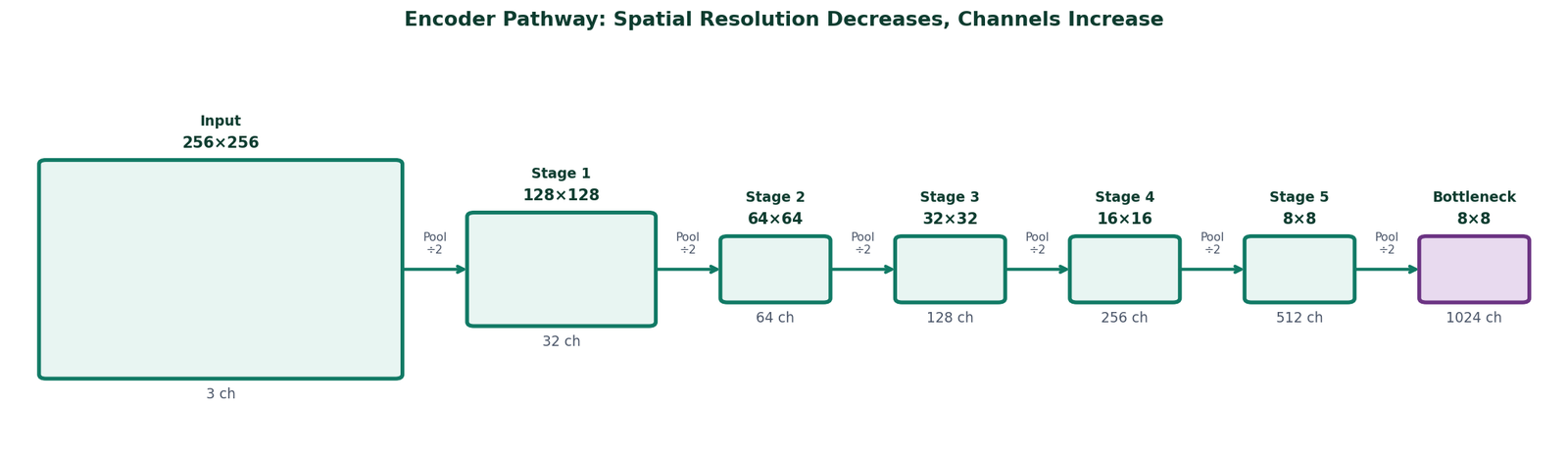
Figure 1 — The encoder pathway. A 256×256 input passes through five downsampling stages, arriving at the bottleneck as an 8×8 feature map with 1024 channels. Spatial resolution shrinks at each stage while channel depth grows, the network trades location precision for semantic understanding.
The encoder is the left half of U-Net. It applies two convolutional layers at each stage, followed by a max-pooling operation that halves the spatial dimensions before the next stage.
For a 256×256 input image, the five-stage encoder used in our CVC-ClinicDB model produces feature maps at the following resolutions:
| Encoder Stage | Feature Map Size | Channels | Receptive Field |
|---|---|---|---|
| Input | 256 × 256 | 3 | 1 pixel |
| Stage 1 output | 256 × 256 | 32 | ~3 × 3 region |
| Stage 2 output | 128 × 128 | 64 | ~6 × 6 region |
| Stage 3 output | 64 × 64 | 128 | ~12 × 12 region |
| Stage 4 output | 32 × 32 | 256 | ~24 × 24 region |
| Stage 5 output | 16 × 16 | 512 | ~32 × 32 region |
| Bottleneck | 8 × 8 | 1024 | ~64 × 64 region |
Notice two things happening simultaneously. The spatial dimensions shrink, from 256×256 to 8×8, while the channel count grows, from 3 to 1024. The network is trading spatial resolution for representational depth. At the bottleneck, each of the 8×8 positions carries a rich 1024-dimensional description of a large region of the original image. It knows what is there. It has lost the fine-grained where.
This is by design, not by accident. The large receptive field at the bottleneck is what allows the network to understand global context, whether the overall image looks like it contains a large central polyp, or scattered small ones, or nothing unusual at all.
The Decoder: Trying to Recover What Was Lost
The decoder is the right half of U-Net. Its job is to take the bottleneck feature map, rich in semantic content but poor in spatial detail and progressively restore spatial resolution until the output matches the original image dimensions.
It does this through transposed convolution operations that reverse the encoder's pooling. At each stage, the feature map is spatially enlarged by a factor of two, and a pair of convolutional layers refines the upsampled features.
But here is the fundamental problem with a decoder operating alone.
Upsampling is not the inverse of downsampling. When max-pooling reduces a region to a single value, it retains the maximum and discards everything else. No upsampling operation can recover what was discarded. The decoder can produce a spatially large output, but that output will be blurry and imprecise at boundaries because the precise boundary information was lost during encoding and cannot be reconstructed from the bottleneck alone.
This is exactly the problem that forced the skip connection into existence.
Skip Connections: The Actual Innovation
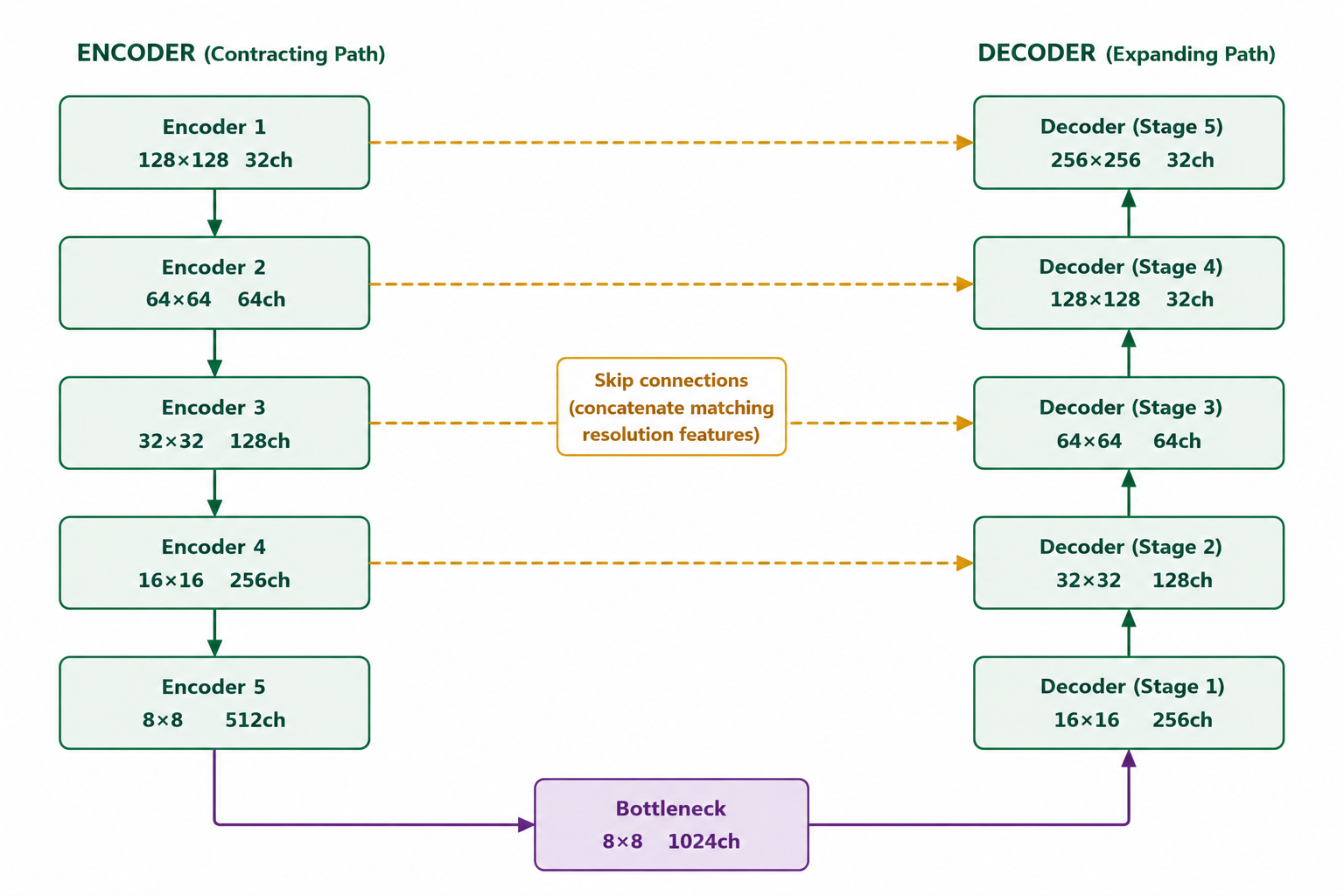
Figure 2 — Skip connections in U-Net. Each encoder stage passes its feature map directly to the corresponding decoder stage at the same spatial resolution. Encoder 1 (128×128) connects to Decoder 5 (128×128), Encoder 2 (64×64) to Decoder 4 (64×64), and so on. The bottleneck feeds into Decoder 1 (8×8), the first decoder stage. Decoder stages then upsample progressively toward the final output.
The skip connection is U-Net's defining contribution. Rather than requiring the decoder to reconstruct fine spatial detail from the bottleneck alone, it gives the decoder direct access to the encoder's feature maps at each spatial scale, before those maps were downsampled.
At each decoder stage, two sources of information are concatenated:
- The upsampled feature map from the previous decoder stage, semantically rich, spatially coarse
- The encoder feature map from the corresponding spatial scale, spatially precise, semantically shallow
The convolutional layers that follow the concatenation learn to integrate these two sources. The semantic information from the decoder path tells the network what the region is. The spatial information from the encoder path tells it exactly where the boundary is.
This is why U-Net produces sharp, precise segmentation boundaries when a decoder-only architecture produces blurry ones. The boundary precision does not come from clever upsampling. It comes from having direct access to the original encoder features that contained that precision before it was lost to downsampling.
Why Concatenation and Not Addition
Skip connections in U-Net use concatenation, the encoder and decoder feature maps are stacked along the channel dimension, doubling the channel count before the next convolution. ResNets use addition instead. The choice matters.
Addition requires the two tensors to have the same meaning for the operation to make sense, you are combining them into a single representation. Concatenation preserves both representations independently and lets the following convolution learn how to use each one. For segmentation, where the encoder and decoder features carry fundamentally different types of information, spatial precision vs semantic depth, concatenation is the right choice.
The Complete Architecture
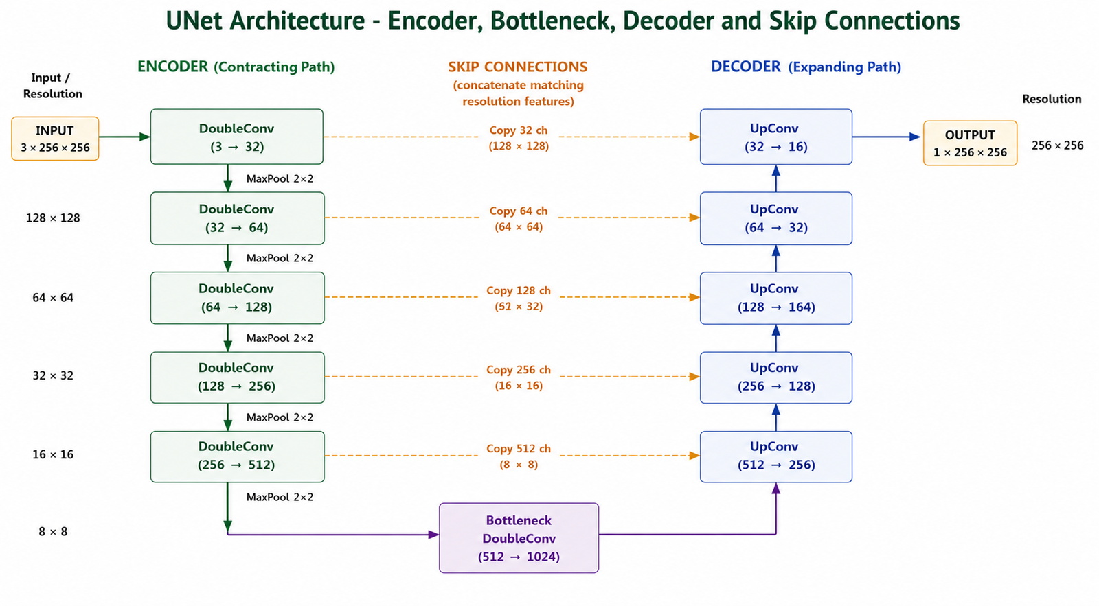
Figure 3 — Complete U-Net architecture as used in the CVC-ClinicDB polyp segmentation experiment. Five encoder stages compress a 256×256 input down to 8×8 at the bottleneck. Five decoder stages restore spatial resolution back to 256×256. Dashed amber arrows show the five skip connections transferring encoder feature maps directly to matching decoder stages. The 1×1 conv with sigmoid at the top of the decoder produces the final binary segmentation mask at full input resolution.
The complete U-Net has a symmetric structure, five encoder stages on the left, a bottleneck at the bottom, five decoder stages on the right, with skip connections bridging each encoder-decoder pair at the same spatial resolution.
The U shape is not an accident of diagram layout. It is a direct consequence of the architecture's function: compress spatial information as you go down, expand it as you go up, and maintain direct connections between the corresponding levels on each side.
Training U-Net on CVC-ClinicDB — What It Actually Looks Like
The model used throughout this post is a U-Net trained from scratch on the CVC-ClinicDB colonoscopy polyp dataset. The channel widths follow the pattern [32, 64, 128, 256, 512] across the five encoder stages, with a 1024-channel bottleneck. The loss function is BCE + Dice combined, which was shown in Blog 1 to produce reliable foreground detection from the first epochs.
class DoubleConv(nn.Module):
    def __init__(self, in_channels, out_channels):
        super().__init__()
        self.conv = nn.Sequential(
            nn.Conv2d(in_channels, out_channels,
                      kernel_size=3, padding=1,
                      bias=False),
            nn.BatchNorm2d(out_channels),
            nn.ReLU(inplace=True),
            nn.Conv2d(out_channels, out_channels,
                      kernel_size=3, padding=1,
                      bias=False),
            nn.BatchNorm2d(out_channels),
            nn.ReLU(inplace=True),
        )

    def forward(self, x):
        return self.conv(x)


class UNET(nn.Module):
    def __init__(self, num_classes=1,
                 input_channels=3, **kwargs):
        super().__init__()
        nb_filter = [32, 64, 128, 256, 512]
        self.pool = nn.MaxPool2d(2, 2)

        # Encoder
        self.conv0_0 = DoubleConv(input_channels, nb_filter[0])
        self.conv1_0 = DoubleConv(nb_filter[0],   nb_filter[1])
        self.conv2_0 = DoubleConv(nb_filter[1],   nb_filter[2])
        self.conv3_0 = DoubleConv(nb_filter[2],   nb_filter[3])
        self.conv4_0 = DoubleConv(nb_filter[3],   nb_filter[4])

        # Bottleneck
        self.bottleneck = DoubleConv(nb_filter[4], nb_filter[4] * 2)

        # Decoder
        self.upconv4 = nn.ConvTranspose2d(nb_filter[4] * 2, nb_filter[4], 2, 2)
        self.conv4_1 = DoubleConv(nb_filter[4] * 2, nb_filter[4])

        self.upconv3 = nn.ConvTranspose2d(nb_filter[4], nb_filter[3], 2, 2)
        self.conv3_2 = DoubleConv(nb_filter[3] * 2, nb_filter[3])

        self.upconv2 = nn.ConvTranspose2d(nb_filter[3], nb_filter[2], 2, 2)
        self.conv2_3 = DoubleConv(nb_filter[2] * 2, nb_filter[2])

        self.upconv1 = nn.ConvTranspose2d(nb_filter[2], nb_filter[1], 2, 2)
        self.conv1_4 = DoubleConv(nb_filter[1] * 2, nb_filter[1])

        self.upconv0 = nn.ConvTranspose2d(nb_filter[1], nb_filter[0], 2, 2)
        self.conv0_5 = DoubleConv(nb_filter[0] * 2, nb_filter[0])

        self.final = nn.Conv2d(nb_filter[0], num_classes, kernel_size=1)

    def forward(self, x):
        x0_0 = self.conv0_0(x)
        x1_0 = self.conv1_0(self.pool(x0_0))
        x2_0 = self.conv2_0(self.pool(x1_0))
        x3_0 = self.conv3_0(self.pool(x2_0))
        x4_0 = self.conv4_0(self.pool(x3_0))
        x5_0 = self.bottleneck(self.pool(x4_0))

        x4_1 = self.conv4_1(
            torch.cat([self.upconv4(x5_0), x4_0], dim=1))
        x3_2 = self.conv3_2(
            torch.cat([self.upconv3(x4_1), x3_0], dim=1))
        x2_3 = self.conv2_3(
            torch.cat([self.upconv2(x3_2), x2_0], dim=1))
        x1_4 = self.conv1_4(
            torch.cat([self.upconv1(x2_3), x1_0], dim=1))
        x0_5 = self.conv0_5(
            torch.cat([self.upconv0(x1_4), x0_0], dim=1))

        return torch.sigmoid(self.final(x0_5))


def criterion(pred, mask):
    return bce_loss(pred, mask) + dice_loss(pred, mask)
What Predictions Look Like at Different Training Stages
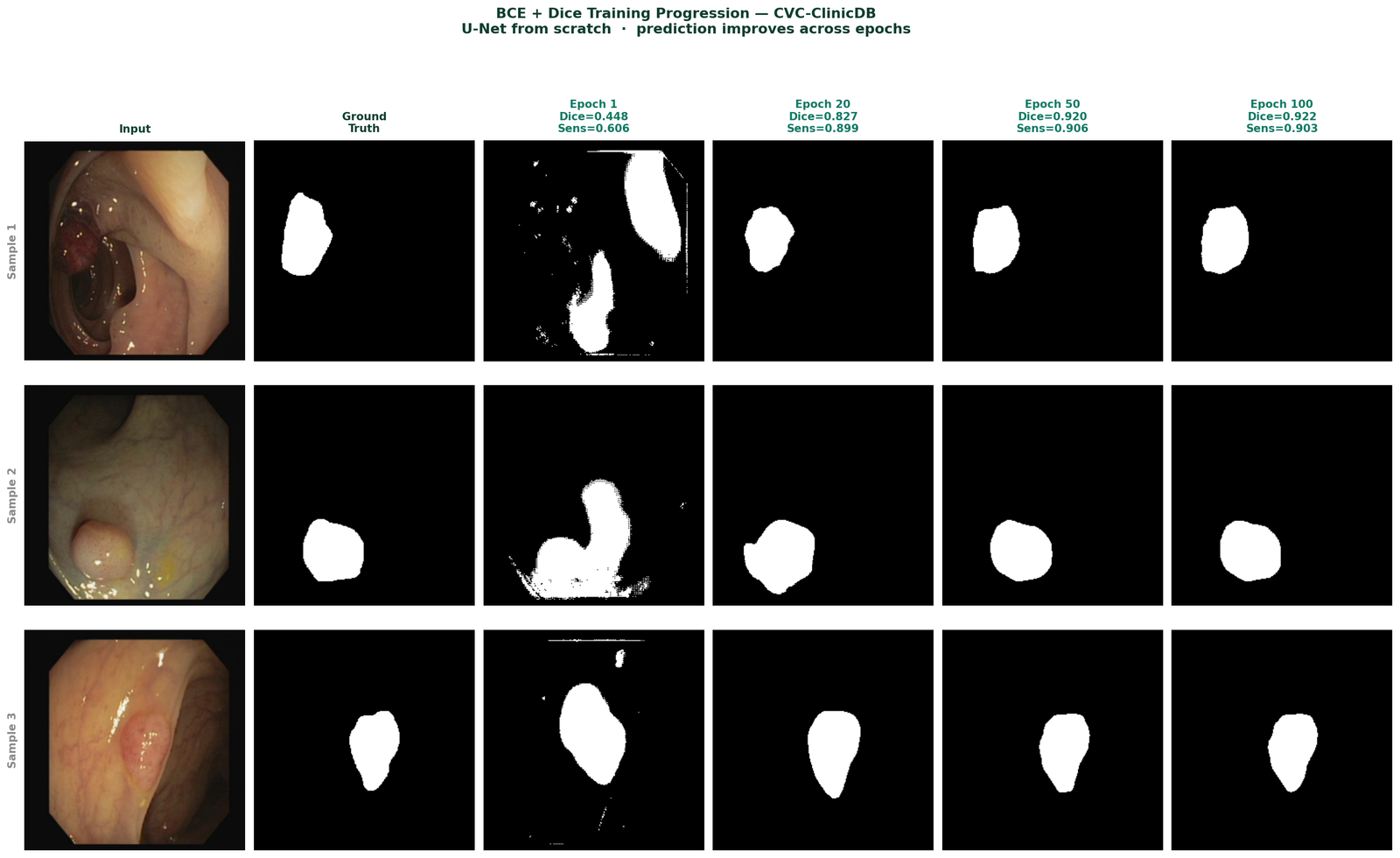
Figure 4 — U-Net predictions on CVC-ClinicDB test images at epochs 1, 20, 50, and 100. Epoch 1: rough initial detection with noisy boundaries and false positives. Epoch 20: recognisable polyp shapes with improved boundaries, Dice 0.827. Epoch 50: clean segmentation, Dice 0.920. Epoch 100: precise boundaries closely matching ground truth, Dice 0.922.
The progression of predictions across epochs reflects what the model is learning in sequence. It learns the global presence of a polyp before it learns its extent, and it learns approximate extent before it learns precise boundaries. The skip connections are what enable the final stage, precise boundaries require the spatial detail that the encoder preserved, and that detail only becomes useful to the decoder after it has learned the semantic context from the bottleneck.
Training Curves

Figure 5 — Validation metrics over 100 training epochs. IoU and Dice converge steadily, reaching best values of 0.8664 and 0.9277 respectively at epoch 80. Sensitivity peaks at 0.9234 at epoch 25. Specificity reaches 0.9959 at epoch 53. All metrics plateau after epoch 60, indicating full convergence.
The training curves confirm the pattern established in Blog 1. BCE + Dice produces reliable sensitivity from the first epochs, the model finds polyps early and refines boundary precision over subsequent epochs. The IoU and Dice curves show steady improvement without collapse, which is the signature of a well-functioning loss function on an imbalanced dataset.
What U-Net Does Not Do Well
Understanding the architecture's limitations is as important as understanding its strengths.
Very small objects. When a polyp occupies only 1 to 2% of the image area, it may be represented by just a handful of pixels at the bottleneck. The global context is dominated by the surrounding healthy tissue. The model has very little signal to work with for objects this small. Higher input resolution and specialized loss functions help, but the fundamental constraint is architectural.
Computational cost at high resolution. The five-stage U-Net with channel widths [32, 64, 128, 256, 512] has approximately 7 million parameters. At 512×512 input, a batch of eight images requires substantial GPU memory. Scaling to higher resolutions quickly hits hardware limits.
Multiscale feature capture at the bottleneck. The standard U-Net bottleneck applies the same double-convolution block used throughout the encoder. It has no dedicated mechanism for capturing contextual information at multiple scales simultaneously, a limitation that more recent architectures address explicitly through modules like ASPP or dilated convolution pyramids.
Selected implementations, supporting utilities, and companion resources related to this article are available through the Blog 3 Companion Resources page .
Companion Resources Included
- U-Net architecture implementation
- DoubleConv block reference
- U-Net training configuration
- Skip connection logic reference
- Training curve plotting utility
- Architecture figure notes
The One Thing to Remember
U-Net works because it gives the decoder direct access to the spatial detail that the encoder preserved before discarding it through downsampling. The skip connections are not a regularization trick or an optimization convenience. They are the solution to a specific, fundamental problem, the irrecoverable loss of spatial information during encoding.
Every modern segmentation architecture that outperforms U-Net does so by addressing one of the limitations listed above, while keeping the core encoder-decoder-skip-connection structure intact. Understanding why U-Net is designed the way it is makes those improvements immediately comprehensible, because you can see exactly which problem each one is solving.
Training a segmentation model and running into issues this post does not cover?
Feel free to reach out through occulinslab.com/contact