You train a segmentation model. Loss decreases. Validation accuracy looks stable. You feel good about where things are heading.
Then you check the actual predictions. Everything is black. No polyps detected. No boundaries. Just empty masks where the objects should be.
Or a more dangerous version of the same problem: the predictions look reasonable after 100 epochs of full training, but if you had stopped at epoch 20, which many practitioners do, especially when time or compute is limited, your model would have been missing 70% of the objects it was supposed to find.
Both of these are symptoms of the same root cause. Understanding it precisely is what allows you to fix it rather than just adjust training until something works.
What Is Actually Happening
In semantic segmentation, the model assigns a class label to every pixel in the image. When the foreground class occupies a small fraction of pixels, the model can achieve high overall accuracy simply by predicting background everywhere. From the perspective of a pixel-wise loss function, this is a perfectly rational solution.
This is what is called a degenerate solution. The model is not broken, it found a local minimum that satisfies the training objective without learning to detect anything useful. The problem is that the training objective did not make foreground detection valuable enough to pull the model out of that minimum.
The Real Cause: Class Imbalance in Your Dataset
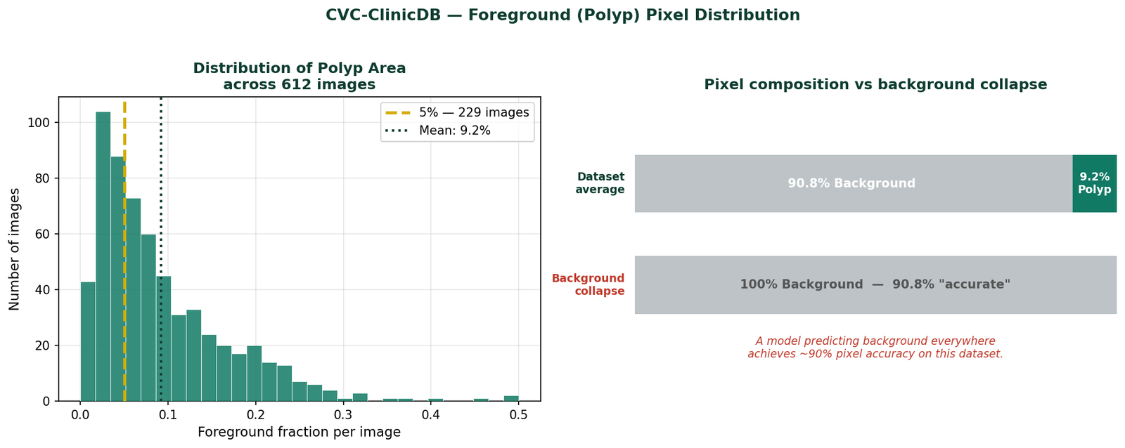
The CVC-ClinicDB colonoscopy dataset has the following pixel distribution across its 612 images:
Mean foreground (polyp):   9.2%
Median foreground:         6.8%
Images below 5% foreground: 229 (37% of dataset)
Images below 10% foreground: 404 (66% of dataset)
At these fractions, a model that predicts background everywhere achieves pixel accuracy of 90 to 93%. That number will appear in your training logs and look completely reasonable. The foreground IoU will be near zero, but if you are only checking overall accuracy, or if your framework reports it prominently, you may not notice until you look at the actual predictions.
Why Cross-Entropy Makes This Worse
Cross-entropy computes the loss at every pixel independently and takes the mean across all pixels. This means the total gradient signal is a weighted average, weighted by pixel count, of the per-pixel gradients. At 9% foreground fraction, background pixels contribute 91% of the gradient and foreground pixels contribute 9%.
The model receives ten times more information about how to classify background than how to classify foreground. It learns background first, fast, and confidently. It learns foreground slowly, noisily, and only after background is fully saturated.
This is not a flaw in cross-entropy. It is exactly how an unweighted average behaves on an imbalanced distribution. The flaw is applying it without modification when the imbalance is this severe.
The Experiment: Two Identical Models, Two Loss Functions
To make this concrete rather than theoretical, I ran two identical experiments on CVC-ClinicDB polyp segmentation. Same model (U-Net trained from scratch with no pretrained weights), same optimizer, same hyperparameters, same 80/20 train-test split with fixed seed. Only the loss function changed.
Experiment A used binary cross-entropy only. Experiment B used BCE combined with Dice loss.

Early Training — Where the Problem Is Most Visible
The sensitivity metric, the fraction of true polyp pixels the model correctly identifies, tells the most important part of the story:
| Epoch | BCE Sensitivity | BCE Specificity | BCE+Dice Sensitivity | BCE+Dice Specificity |
|---|---|---|---|---|
| 1 | 0.424 | 0.896 | 0.606 | 0.906 |
| 2 | 0.268 | 0.981 | 0.684 | 0.918 |
| 5 | 0.541 | 0.982 | 0.795 | 0.971 |
| 10 | 0.747 | 0.986 | 0.889 | 0.951 |
| 20 | 0.850 | 0.990 | 0.899 | 0.975 |
| 30 | 0.899 | 0.992 | 0.913 | 0.990 |
Look at epoch 2. BCE sensitivity drops to 0.268 while BCE specificity climbs to 0.981. The model is predicting background with increasing confidence, exactly the degenerate solution described above. BCE + Dice shows sensitivity of 0.684 at the same epoch. It is finding polyps from the very start because the Dice component makes foreground detection non-negotiable for the loss.
By epoch 10, BCE has recovered somewhat to 0.747 sensitivity, but BCE + Dice is already at 0.889. The gap is 14 percentage points at epoch 10, and it does not close until around epoch 30 to 40.
Final Results at Epoch 100
| Configuration | Best Dice | Final IoU | Final Sensitivity | Final Specificity |
|---|---|---|---|---|
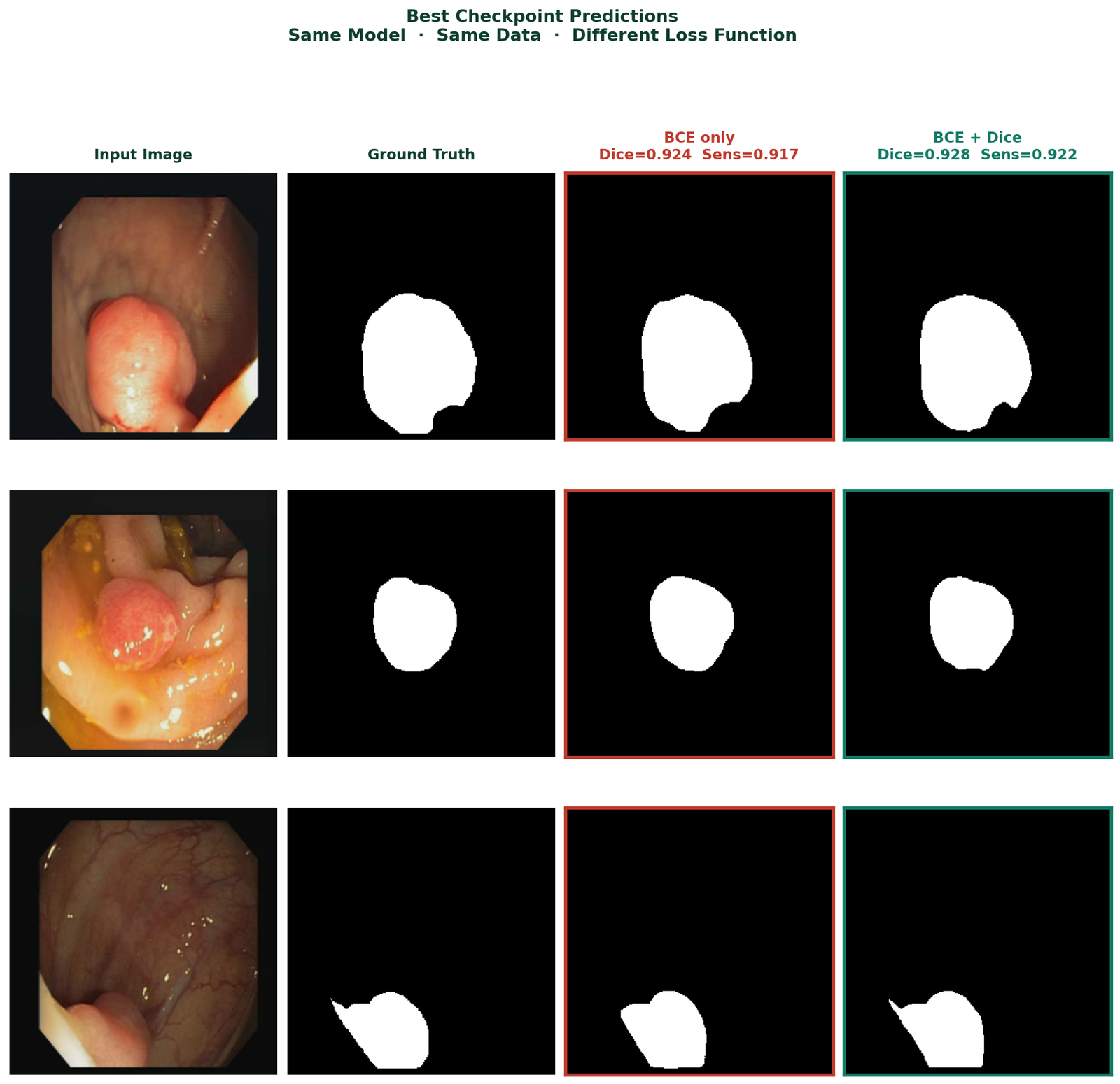
| BCE only | 0.9245 | 0.8508 | 0.9177 | 0.9929 |
| BCE + Dice | 0.9277 | 0.8574 | 0.9220 | 0.9951 |
At full convergence after 100 epochs, the two models reach similar performance. BCE + Dice has slightly higher Dice and IoU. BCE only has slightly higher final sensitivity, though it took 30 epochs longer to get there. Both are viable at epoch 100. The question is what happens if you stop earlier, and what happens during the 30 epochs where BCE is still catching up.
The Fix: Combined BCE and Dice Loss
The single most effective change is replacing cross-entropy alone with a combination of BCE and Dice loss. The code is straightforward:
import torch
import torch.nn as nn

class DiceLoss(nn.Module):
    def __init__(self, eps=1.0):
        super().__init__()
        self.eps = eps

    def forward(self, pred, target):
        # pred is already sigmoid-activated
        num   = 2 * (pred * target).sum() + self.eps
        denom = pred.sum() + target.sum() + self.eps
        return 1 - num / denom

bce_loss  = nn.BCELoss()
dice_loss = DiceLoss()

def criterion(pred, mask):
    return bce_loss(pred, mask) + dice_loss(pred, mask)
BCE provides stable gradients throughout training particularly important in early epochs when predictions are still near random. Dice ensures the foreground class cannot be overwhelmed by the background gradient signal. Together they are consistently more robust than either alone on imbalanced segmentation tasks.
One note on implementation: if your model applies torch.sigmoid internally in its forward method, as many U-Net implementations do, use nn.BCELoss which expects probabilities in [0, 1]. If your model outputs raw logits, use nn.BCEWithLogitsLoss which applies sigmoid internally. Mixing these causes double-sigmoiding which produces near-uniform outputs and very small gradients throughout training.
Before You Change the Loss: Diagnose First
Not every blank prediction is a loss function problem. Before changing your training configuration, verify these three things.
Is your model actually in foreground collapse?
After 20 epochs, compute foreground IoU and sensitivity specifically, not overall pixel accuracy. Foreground IoU below 0.10 combined with overall accuracy above 88% is the signature of foreground underweighting. Overall accuracy above 90% on a dataset with 9% foreground is a warning sign, not a success signal.
Are your masks correct?
Open five random image-mask pairs and look at them directly. Confirm the masks contain the objects you expect, that they are not inverted, and that filenames sort in the same order for images and masks. Mismatched pairs are more common than expected and they corrupt the training signal silently.
Are your mask values what you think they are?
import numpy as np
from PIL import Image
import os

mask_dir = 'CVC-ClinicDB/masks'

for fname in sorted(os.listdir(mask_dir))[:5]:
    mask = np.array(
        Image.open(
            os.path.join(mask_dir, fname)
        ).convert('L')
    )
    fg = (mask > 127).sum() / mask.size
    print(f"{fname}: unique={np.unique(mask)} "
          f"fg_fraction={fg:.4f}")
Binary masks should have values 0 and 255 (before normalisation) or 0.0 and 1.0 (after). If unique values return something unexpected, all zeros, all 255, or a range of intermediate values, fix the mask loading before adjusting anything else.
Monitoring Predictions During Training
Do not wait until epoch 100 to look at predictions. Save a prediction image at fixed intervals during training:
def save_prediction_sample(model, loader, epoch,
                            save_dir, device):
    model.eval()
    os.makedirs(save_dir, exist_ok=True)
    with torch.no_grad():
        images, masks = next(iter(loader))
        images = images.to(device)
        preds  = model(images)
        pred_mask = (preds[0].cpu().squeeze() > 0.5
                     ).float().numpy()
    fig, axes = plt.subplots(1, 3, figsize=(10, 3))
    axes[0].imshow(images[0].cpu().permute(1,2,0))
    axes[0].set_title('Input'); axes[0].axis('off')
    axes[1].imshow(masks[0].squeeze(), cmap='gray')
    axes[1].set_title('Ground Truth'); axes[1].axis('off')
    axes[2].imshow(pred_mask, cmap='gray')
    axes[2].set_title(f'Epoch {epoch}'); axes[2].axis('off')
    plt.tight_layout()
    plt.savefig(f'{save_dir}/epoch_{epoch:03d}.png', dpi=120, bbox_inches='tight')
    plt.close()
    model.train()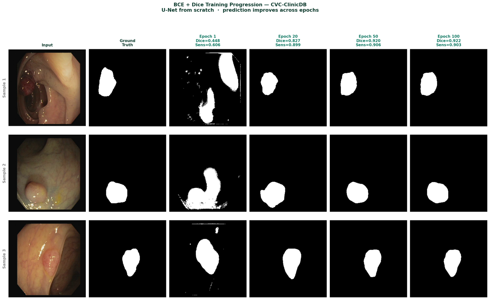
The One Metric That Reveals Foreground Collapse
Sensitivity, the fraction of true foreground pixels correctly identified, is the metric that exposes this failure mode most clearly. Always track foreground sensitivity alongside your primary metrics. For binary medical segmentation especially, it is the number that tells you whether the model is clinically useful or not.
Summary
| Symptom | Cause | Fix |
|---|---|---|
| All-black predictions | Complete foreground collapse under BCE | Replace with BCE + Dice combined loss |
| Low sensitivity in early training | BCE gradient dominated by background pixels | BCE + Dice — Dice component protects foreground signal |
| Good accuracy, poor IoU | Model predicting background accurately | Report foreground IoU and sensitivity, not overall accuracy |
| Training looks normal, predictions wrong | Wrong activation-loss pairing | Match BCELoss to sigmoid model, BCEWithLogitsLoss to logit model |
| Cannot tell what is happening | Only tracking aggregate metrics | Visualize predictions every 10 epochs, track sensitivity separately |
The pattern in this experiment is consistent across datasets with moderate to severe foreground imbalance. BCE + Dice does not always produce dramatically higher final metrics after full convergence. What it consistently produces is faster, more reliable foreground detection, particularly in the first 30 epochs where BCE is still learning to find the foreground at all.
Selected implementations, supporting utilities, experiment configurations, and companion resources related to this article are available through the Blog 1 Companion Resources page .
Companion Resources Included
- U-Net architecture implementation
- Dice Loss implementation
- BCE + Dice combined loss function
- Metric calculation utilities
- Prediction visualization utilities
- Foreground imbalance inspection utilities
- Example experiment configuration
Working on segmentation systems where metrics and predictions do not align?
Reach out through
Occulins Contact
for deployment-aware computer vision research and engineering support.