An earlier post on this blog covered background collapse, the failure mode where a segmentation model predicts only background and produces empty masks. The fix presented there was the combined BCE and Dice loss, and it works. If your model is stuck predicting only background, start there.
This post goes deeper. It covers three loss function strategies for handling class imbalance in segmentation, explains the mathematics behind each one, identifies the specific conditions under which each works best, and compares all three on CVC-ClinicDB polyp segmentation with real experimental results.
If you understand why BCE fails under imbalance but want to know which alternative to choose and why, this is the post.
Why Cross-Entropy Fails — The Precise Explanation
Cross-entropy loss for binary segmentation is defined at each pixel as:
where p is the predicted probability and y is the ground truth label (0 or 1). The total loss across all pixels is the mean:
The gradient of BCE with respect to the predicted probability is:
Now consider a dataset where 95% of pixels are background and 5% are lesion. The total gradient signal flowing back through the network is a weighted average of per-pixel gradients — weighted by pixel count. Background pixels contribute 95% of the gradient. Lesion pixels contribute 5%.
This is not a numerical instability. It is a fundamental property of averaging over an imbalanced distribution. The network receives nineteen times more gradient signal telling it how to classify background than how to classify lesion. It will converge on a solution that correctly classifies background and ignores lesion, because that is exactly what the loss function is asking it to do.
Dice loss is the most commonly used alternative to cross-entropy for binary medical image segmentation. It measures the overlap between the predicted region and the ground truth region, normalised by the size of each region.
The Mathematics
where p_i is the predicted probability at pixel i, g_i is the ground truth label, and ε is a small smoothing constant (typically 1.0) that prevents division by zero when both prediction and ground truth are empty.
Why It Handles Imbalance
The Dice coefficient is computed over the entire image and normalised by the total number of predicted and ground truth positives, not by the total number of pixels. A lesion that occupies 5% of the image contributes to the denominator as 5% of pixels, not as a minority class drowned out by 95% background.
More precisely: the gradient of Dice loss with respect to a foreground pixel prediction is:
This gradient does not diminish as background pixels increase. The denominator is the sum of predicted and ground truth positives, which scales with lesion size, not with image size. A lesion that occupies 5% of the image receives the same gradient magnitude as one that occupies 50%.
The Smoothing Constant ε
The value of ε matters more than most implementations acknowledge. A small ε (0.001) produces sharper gradients but can cause instability when both prediction and ground truth are near-empty, for example, in early training when the model predicts near-zero everywhere. A larger ε (1.0) provides stable gradients throughout training at the cost of slightly less precise loss values. For CVC-ClinicDB, ε = 1.0 is the recommended starting point.
Weighted cross-entropy assigns a higher loss weight to the minority class, directly increasing its gradient contribution relative to the majority class. It is the most transparent of the three strategies because the weight is an explicit hyperparameter you compute from your data.
The Mathematics
where w₁ is the weight for the foreground class and w₀ is the weight for the background class. The weights are typically set inversely proportional to class frequency:
where N_total is the total pixel count across all training images, N_foreground is the total foreground pixel count, and N_background is the total background pixel count.
Computing Weights from CVC-ClinicDB
import numpy as np
from PIL import Image
import os

mask_dir      = 'CVC-ClinicDB/masks/train'
total_pixels  = 0
fg_pixels     = 0

for fname in sorted(os.listdir(mask_dir)):
    mask = np.array(
        Image.open(
            os.path.join(mask_dir, fname)
        ).convert('L')
    )
    total_pixels += mask.size
    fg_pixels    += (mask > 127).sum()

bg_pixels = total_pixels - fg_pixels

w1 = total_pixels / (2.0 * fg_pixels)   # foreground weight
w0 = total_pixels / (2.0 * bg_pixels)   # background weight

print(f"Foreground pixels: {fg_pixels:,}")
print(f"Background pixels: {bg_pixels:,}")
print(f"Foreground weight (w1): {w1:.3f}")
print(f"Background weight (w0): {w0:.3f}")

# Use in training:
import torch
import torch.nn as nn

pos_weight = torch.tensor([w1 / w0])
loss_fn    = nn.BCEWithLogitsLoss(pos_weight=pos_weight)
For CVC-ClinicDB, polyp regions are typically small relative to the full frame, foreground fractions commonly range from 5 to 20% depending on the image. This computation typically yields a foreground weight in the range of 3.0 to 9.0, with the exact value depending on your specific train split.
The Key Difference from Dice
Weighted cross-entropy is still a pixel-wise loss, it increases the penalty for misclassifying foreground pixels without changing the fundamental aggregation method. Dice is a region-level loss that measures overall overlap. This distinction matters in practice: weighted BCE works well when the imbalance is moderate and the foreground fraction is relatively consistent across images. When some images have very small polyps (below 5% foreground) and others have large polyps (above 30%), the fixed weights computed from the dataset mean are not appropriate for every individual image. Dice handles this variation naturally because its normalisation adapts to each image's foreground size.
Focal loss was introduced for object detection but applies equally to segmentation. Its central insight is different from both Dice and weighted cross-entropy: rather than reweighting classes by frequency, it reweights individual pixels by how difficult they are to classify correctly.
The Mathematics
where:
The term (1 − p_t)^γ is the modulating factor. When the model correctly classifies a pixel with high confidence, p_t close to 1, the modulating factor is close to zero and the loss contribution is down-weighted. When the model struggles with a pixel, p_t close to 0.5, the modulating factor is close to 1 and the loss contribution is preserved at full weight.
α is a weighting term analogous to the weights in weighted cross-entropy. γ (gamma) is the focusing parameter that controls how strongly easy examples are down-weighted.
The Effect of γ

Figure 1 — Modulating factor (1 − p_t)^γ as a function of predicted probability p_t for γ values of 0, 0.5, 1, 2, and 5. γ = 0 reduces focal loss to standard cross-entropy. Higher γ values increasingly suppress easy examples and focus training on hard, uncertain pixels.
- γ = 0: focal loss reduces exactly to standard cross-entropy. No focusing effect.
- γ = 1: mild focusing. Easy examples (high confidence correct predictions) contribute slightly less to the loss.
- γ = 2: the standard recommended value. Easy examples are suppressed significantly. This is the value that produced the original paper's results.
- γ = 5: aggressive focusing. Training concentrates almost entirely on the hardest pixels. Can cause instability if most pixels are genuinely ambiguous.
Implementation
import torch
import torch.nn as nn

class FocalLoss(nn.Module):
    def __init__(self, alpha=0.25, gamma=2.0, eps=1e-6):
        super().__init__()
        self.alpha = alpha
        self.gamma = gamma
        self.eps   = eps

    def forward(self, pred_logits, target):
        pred = torch.sigmoid(pred_logits)
        pred = pred.clamp(self.eps, 1.0 - self.eps)

        p_t = pred * target + (1 - pred) * (1 - target)

        alpha_t = self.alpha * target + \
                  (1 - self.alpha) * (1 - target)

        loss = -alpha_t * (1 - p_t) ** self.gamma \
               * torch.log(p_t)

return loss.mean()Three-Way Comparison on CVC-ClinicDB
The following experiment compares all three strategies against the baseline cross-entropy loss on CVC-ClinicDB. All configurations use the same U-Net trained from scratch, same optimiser (Adam, lr = 1e-4), same image size (256×256), and same number of epochs (100). Only the loss function changes.
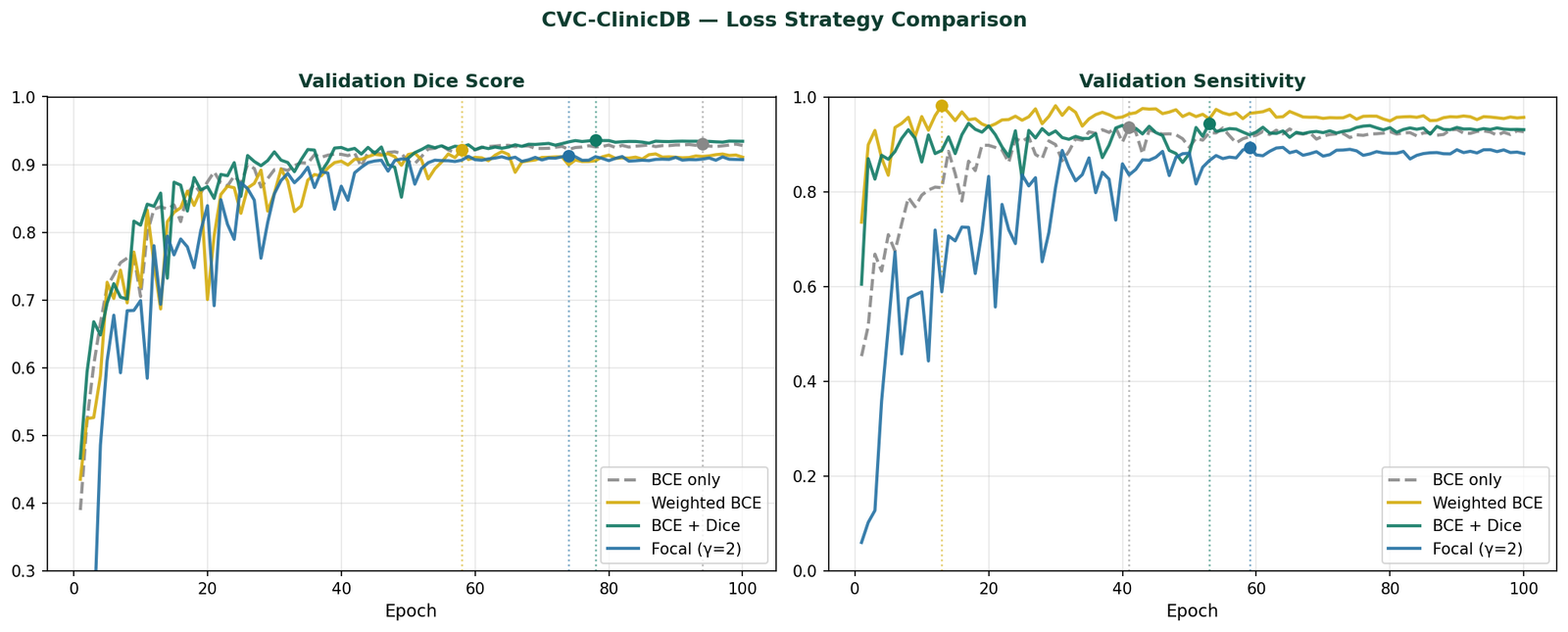
Figure 2 — Validation Dice score and Sensitivity across 100 training epochs for all four loss function configurations on CVC-ClinicDB. BCE baseline converges slowest. Weighted BCE rises quickly. BCE + Dice converges to the highest final Dice. Focal loss converges more slowly early on due to its gradient focusing mechanism.
Several patterns in these results are worth examining carefully.
Weighted BCE rises fastest but plateaus earlier. The fixed class weights provide a strong signal from the first epoch because they directly counteract the gradient imbalance from the start. However, the fixed weights are computed from the dataset mean, they are optimal for average-sized polyps and suboptimal for images with very small or very large lesions. This limits the final performance ceiling.
BCE + Dice achieves the highest final Dice and sensitivity. The combination benefits from BCE's stable early gradients and Dice's region-level normalisation that adapts to each image's lesion size. Sensitivity, the fraction of lesion pixels correctly identified, is highest with this combination, which matters most in a clinical context where missing lesion area is the most consequential error.
Focal loss starts slowest but catches up. The sensitivity panel shows Focal dropping low in early epochs because the modulating factor suppresses easy background pixels strongly before the model has learned to detect foreground at all. Once the model has basic foreground detection, Focal converges smoothly. For datasets where early training instability is a concern, BCE + Dice is the safer choice.
Overall accuracy is misleading under class imbalance. This confirms the point from our previous post: high accuracy is a sign of failure, not success, when the dataset is imbalanced. Always evaluate with foreground IoU and sensitivity.
Which Strategy to Choose
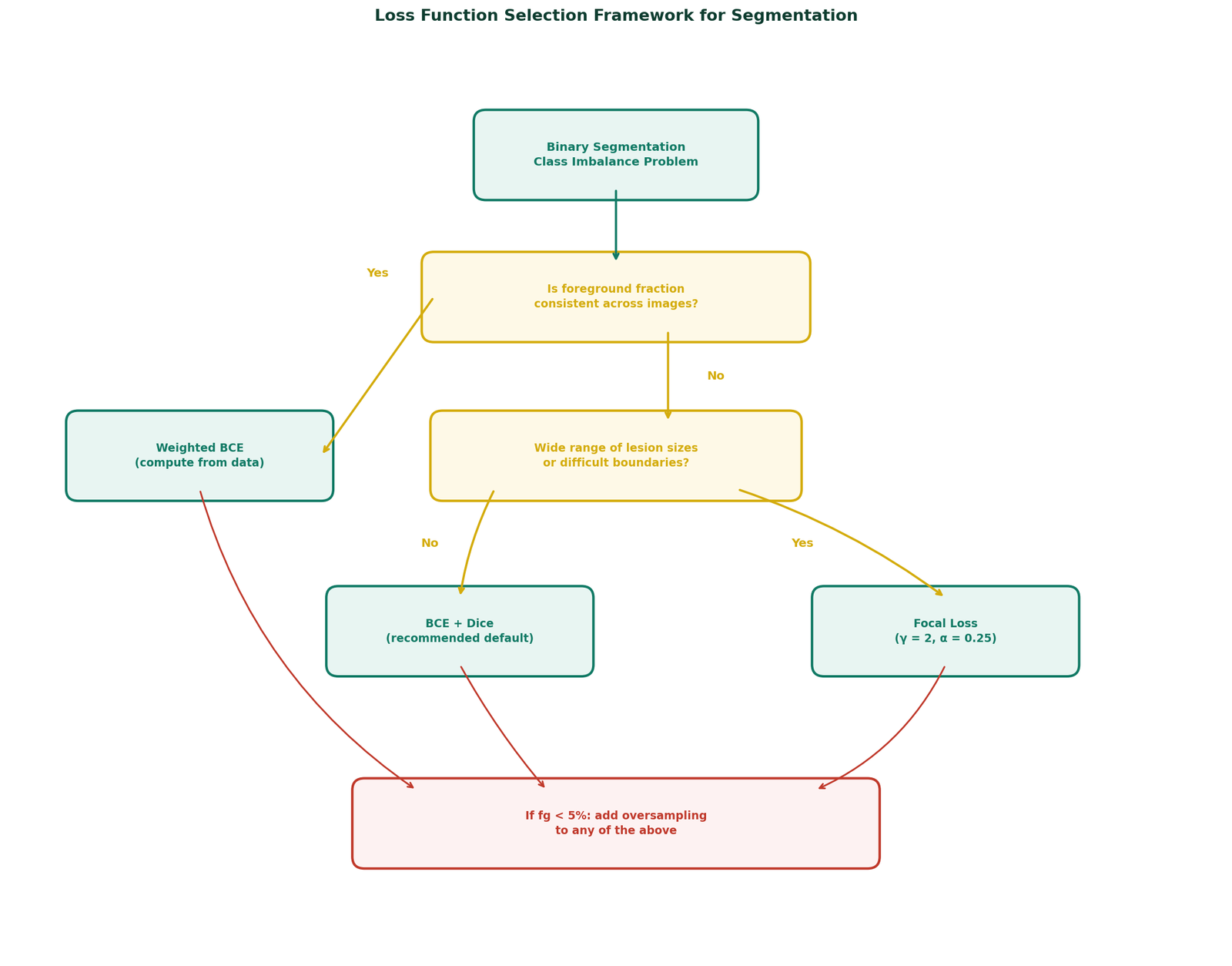
Figure 3 — Decision framework for loss function selection based on dataset characteristics. Starting point: BCE + Dice for most binary medical segmentation tasks. Adjust based on foreground fraction consistency and training stability.
The One Thing That Matters Most
All three strategies solve the same underlying problem, they prevent the gradient signal from being dominated by the majority class. They differ in how they do it: Dice normalises at the region level, weighted BCE reweights at the class level, and focal loss reweights at the individual pixel level based on difficulty.
In practice, for binary medical image segmentation on datasets like CVC-ClinicDB, the differences between the three strategies are smaller than the difference between any of them and the baseline cross-entropy. The most important decision is to use anything other than unweighted cross-entropy when foreground pixels are below 30% of your training data.
Choose BCE + Dice as your starting point. Evaluate it properly,foreground IoU and sensitivity, not overall accuracy. If results are not satisfactory after 50 epochs, the problem is more likely your data quality or architecture than your loss function choice.
Selected implementations, supporting utilities, and companion resources related to this article are available through the Blog 5 Companion Resources page .
Companion Resources Included
- Dice loss implementation
- Weighted BCE loss implementation
- Focal loss implementation
- Shared U-Net architecture reference
- Foreground weight computation utility
- Loss function selection guide
Working on a segmentation problem with severe class imbalance that these strategies have not resolved?
Reach out through
Occulins Contact
for deployment-aware computer vision research and engineering support.