By Dr. Somaiya Khan | Occulins
August 30, 2026
Here is a situation that happens more often than it should. Two segmentation models trained on the same dataset. Model A reports higher mIoU. Model B reports higher Dice. You need to pick one for deployment. Which is better?
If you cannot answer that without more information, this post is for you.
IoU, Dice, and mIoU measure related but distinct properties of segmentation quality. Understanding what each one captures and more importantly what each one hides is what allows you to choose the right metric for your task rather than just reporting whichever number looks best.
A previous post covered IoU in the context of object detection , bounding box overlap and its role in computing mAP. This post covers pixel-level IoU, Dice, and mIoU specifically for semantic segmentation, where the questions are different. A separate post covered Dice loss as a training objective. Here we treat Dice as an evaluation metric, the same formula applied to a different purpose.
Per-Class IoU, The Foundation
In semantic segmentation, IoU is computed at the pixel level for each class separately. For a given class c, every pixel in the image is one of four things:
- True Positive (TP): predicted class c, ground truth class c
- False Positive (FP): predicted class c, ground truth not class c
- False Negative (FN): predicted not class c, ground truth class c
- True Negative (TN): predicted not class c, ground truth not class c
Notice that TN does not appear in the IoU formula. Background pixels that are correctly classified as background contribute nothing to IoU. This is a deliberate and important property. It means IoU measures only the quality of the foreground prediction, not how well the model ignores background. This is why IoU is appropriate for segmentation evaluation even when background dominates the image.
A Worked Example
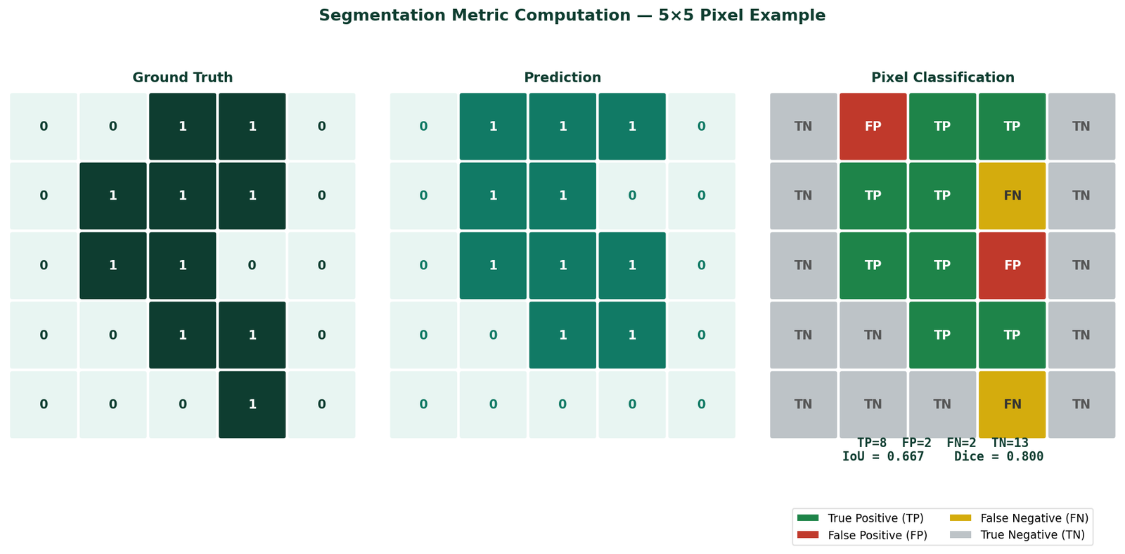
Figure 1 — 5×5 pixel grid showing ground truth (left) and model prediction (centre) for a binary segmentation task. Pixels are colour-coded in the classification panel (right): green = True Positive, red = False Positive, amber = False Negative, grey = True Negative. TP=8, FP=2, FN=2, TN=13. IoU = 8/(8+2+2) = 0.667. Dice = 2×8/(2×8+2+2) = 0.800.
Predicted lesion pixels: 10 (positions where Pred=1)
True Positives (TP): 8 — predicted lesion, is lesion
False Positives (FP): 2 — predicted lesion, is background
False Negatives (FN): 2 — predicted background, is lesion
True Negatives (TN): 13 — predicted background, is background
IoU = TP / (TP + FP + FN) = 8 / (8 + 2 + 2) = 8/12 = 0.667
Dice = 2×TP / (2×TP + FP + FN) = 16 / (16 + 2 + 2) = 16/20 = 0.800
Both metrics agree that the prediction quality is good, above 0.5 on IoU and 0.8 on Dice. But the numbers are different: IoU gives 0.667 and Dice gives 0.800. This is not a discrepancy, it is a fundamental property of how the two formulas weight the same underlying counts.
Dice Score — The Relationship to IoU
The Dice score (also called the F1 score at pixel level) is defined as:
Comparing the two formulas side by side reveals the mathematical relationship:
This relationship has two important consequences.
First: IoU and Dice always agree on ranking. If Model A has higher IoU than Model B for the same class on the same dataset, it will also have higher Dice. The two metrics cannot contradict each other on ranking, they are monotonically related. The scenario in the opening paragraph with Model A higher IoU, and Model B higher Dice, cannot happen for the same class. It can only happen when the two models are compared on different classes or when mIoU vs mean Dice are compared across a multi-class dataset with different class distributions.
Second: Dice is always higher than IoU for the same prediction. Because Dice = 2×IoU / (1 + IoU) and IoU is always between 0 and 1, Dice is always closer to 1 than IoU for any non-perfect prediction. At IoU = 0.5, Dice = 0.667. At IoU = 0.75, Dice = 0.857. At IoU = 1.0, both equal 1.0.

Figure 2 — Dice score as a function of IoU across the range 0 to 1. The curve shows that Dice is always higher than IoU for any intermediate prediction quality. At perfect overlap (IoU=1) both metrics equal 1.0. At no overlap (IoU=0) both equal 0.0. The shaded region illustrates how much Dice exceeds IoU at each quality level. Annotated points: IoU=0.30→Dice=0.462, IoU=0.50→Dice=0.667, IoU=0.75→Dice=0.857.
Why Dice Appears More Generous
Dice double-weights true positives in the numerator (2×TP) relative to IoU (TP). This makes Dice more sensitive to the overlap between prediction and ground truth and less sensitive to the total extent of disagreement. In practical terms, a model that gets most of the lesion right but misses some edges will score higher on Dice than IoU because the overlap it does achieve is counted more strongly relative to the errors.
Neither weighting is inherently correct. The choice between IoU and Dice as the primary evaluation metric should reflect what you care about in your application.
Mean IoU — What It Aggregates and What It Hides
For multi-class segmentation, per-class IoU is computed separately for each class and then averaged. This average is mIoU, the standard benchmark metric for semantic segmentation.
mIoU treats every class equally regardless of how frequently it appears in the dataset. A class that appears in 1% of images contributes as much to mIoU as a class that appears in 99% of images. This equal weighting is intentional and appropriate for benchmarking as it prevents a model from gaming the metric by focusing on the most common classes.
The Problem: mIoU Hides Per-Class Failure
Mucosa: IoU = 0.85 — common tissue class, well learned
Polyp: IoU = 0.74 — target lesion class
Instrument: IoU = 0.07 — rare class, near-complete failure
mIoU = (0.96 + 0.85 + 0.74 + 0.07) / 4 = 0.655
A published mIoU of 0.655 sounds competitive. But the model is detecting surgical instruments with IoU of 0.07 — essentially failing completely on a clinically critical class. The aggregate number hides this completely.
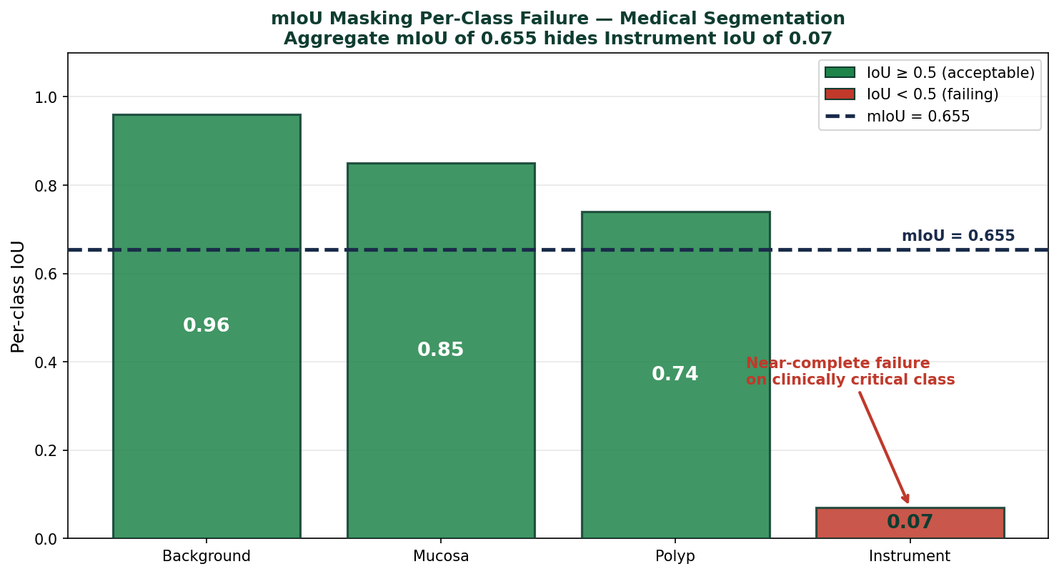
Figure 3 — Per-class IoU for a four-class medical segmentation model alongside the mIoU aggregate. The mIoU of 0.655 appears competitive. The per-class breakdown reveals that Instrument IoU is 0.07 which is near-complete failure on a clinically critical class. The dashed line shows the mIoU reference across all classes.
This is the central limitation of mIoU. The equal class weighting that makes it a fair benchmark metric is the same property that allows a catastrophic per-class failure to be invisible in the aggregate.
The practical implication is direct: always look at per-class IoU alongside mIoU. In any framework, per-class IoU is available in the detailed validation output even when mIoU is the headline number. Read it every time.
When IoU and Dice Give Different Signals
Since IoU and Dice are monotonically related, they cannot contradict each other for a single class prediction. But there are two situations where they give genuinely different information.
Situation 1: Comparing Models Across Imbalanced Classes
When computing mean Dice across classes, the equal weighting is the same as mIoU — each class contributes equally. But because Dice is more generous than IoU for intermediate prediction quality, mean Dice always exceeds mIoU by a varying amount that depends on the specific prediction quality distribution.
If Model A has stronger performance on a rare hard class and Model B has stronger performance on common easy classes, the two models can rank differently on mIoU versus mean Dice not because the metrics disagree about any individual class, but because the non-linear relationship between them magnifies differences at certain quality levels.
| Class | Model A IoU | Model B IoU | Model A Dice | Model B Dice |
|---|---|---|---|---|
| Class 1 (common) | 0.90 | 0.95 | 0.947 | 0.974 |
| Class 2 (rare) | 0.60 | 0.40 | 0.750 | 0.571 |
| Mean | 0.750 | 0.675 | 0.849 | 0.773 |
In this example both mIoU and mean Dice agree that Model A is better, IoU 0.750 vs 0.675, Dice 0.849 vs 0.773. But the magnitude of the difference looks larger in Dice because Dice amplifies the gap at the intermediate quality levels where the rare class sits. Reporting Dice alone makes Model A look substantially better than it is relative to Model B. Reporting IoU gives a more conservative and more informative picture of the actual quality gap.
Situation 2: Sensitivity vs Precision Trade-off
IoU penalises both false positives and false negatives equally — they both appear in the denominator with equal weight. Dice also penalises both equally. Neither metric explicitly rewards sensitivity (finding all the true lesion) over precision (not labelling background as lesion).
However, in clinical applications these two error types have different costs. A missed lesion (false negative) in polyp detection has a higher cost than a false alarm (false positive). Neither IoU nor Dice captures this asymmetry, for that you need to compute sensitivity and specificity separately alongside the overlap metrics.
Which Metric to Report When
mIoU — report for benchmarking and comparison with literature
mIoU is the standard metric for semantic segmentation benchmarks. If you are comparing against published results, mIoU is what the literature reports and what reviewers expect. It is the right metric for demonstrating that your model is competitive.
Per-class IoU — report for understanding model behaviour
Per-class IoU reveals where the model fails. It is the diagnostic metric that mIoU hides. Any evaluation that informs a deployment decision should include per-class IoU — not just the mean.
Dice — report for medical imaging and clinical audiences
Dice (F1) is more familiar to clinical collaborators than IoU and is the metric most commonly reported in medical image segmentation papers. It is mathematically equivalent to IoU for ranking purposes but gives higher numerical values that are easier to communicate to non-technical stakeholders. For binary medical segmentation tasks, reporting both Dice and IoU is standard practice.
Sensitivity — report for clinical safety-critical applications
When the cost of missing a true positive is higher than the cost of a false positive which is almost always the case in polyp and lesion detection, sensitivity must be reported separately. IoU and Dice do not distinguish between these error types. Sensitivity does.
The Three Things Most Practitioners Get Wrong
Reporting only mIoU without per-class breakdown. The aggregate hides failures that matter. A model with mIoU of 0.72 may be failing catastrophically on one class. Read the per-class table every time you run validation.
Treating Dice as more accurate than IoU because the number is higher. Dice is not more accurate, it is more generous. The higher number reflects the mathematical relationship between the formulas, not superior prediction quality. A model with Dice of 0.85 and a model with IoU of 0.74 may be the exact same model because Dice(IoU=0.74) = 2×0.74/(1+0.74) = 0.85.
Omitting sensitivity from medical segmentation evaluation. In clinical contexts, sensitivity is the number that matters most as it measures whether the model finds the pathology. IoU and Dice measure prediction overlap. They are not the same thing and they are not interchangeable for clinical decision-making.
Selected implementations, supporting utilities, and companion resources related to this article are available through the Blog 8 Companion Resources page .
Companion Resources Included
- Segmentation metrics function (per-class IoU, Dice, sensitivity, specificity, mIoU)
Working on a segmentation task and uncertain which evaluation approach is right for your application?
Reach out through
Occulins Contact
for deployment-aware computer vision research and engineering support.