Most object detection tutorials follow the same pattern.
Install the framework. Download a pre-prepared dataset. Run the training command. Look at the predictions. Done.
That pattern works perfectly for the tutorial. It almost never works for your actual dataset.
The gap between running a tutorial successfully and training a model on your own data is where most people get stuck, and it is not because they are missing a command or a library. It is because tutorials teach you the steps, not the decisions. And in object detection, the decisions are what determine whether your model learns anything useful.
This post covers those decisions. We will use YOLOv12 trained on the VisDrone dataset as the running example throughout, VisDrone is an aerial drone detection dataset with real challenges that make the decisions matter, which is exactly what we need to learn from.
Why VisDrone and Why YOLOv12
VisDrone is a drone-captured dataset for detecting pedestrians, cars, vans, trucks, bicycles, and other objects in aerial imagery. It has roughly 6,500 training images and 548 validation images, with objects that are small, densely packed, and photographed from varying altitudes.
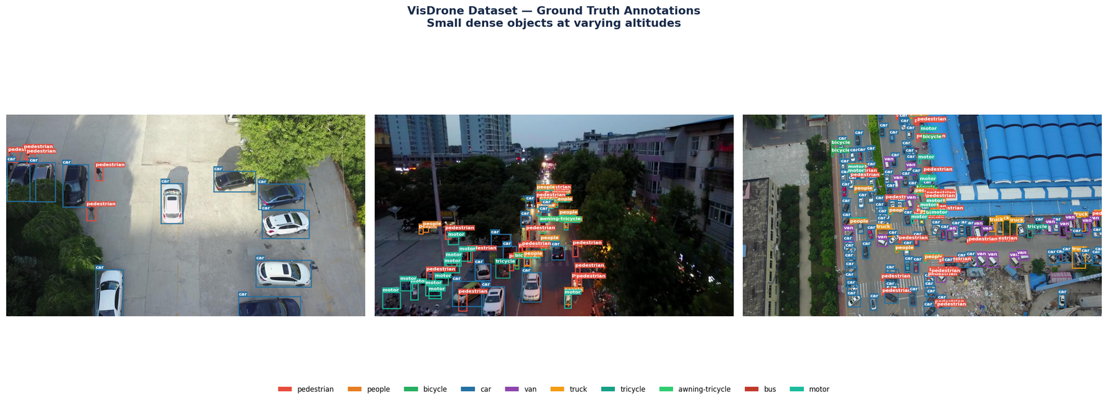
Figure 1 — Three sample VisDrone validation images with ground truth annotations. Left: sparse parking lot scene with cars and pedestrians at moderate altitude. Centre: dense night-time street scene with motors, tricycles, and pedestrians. Right: high-altitude view with hundreds of densely packed objects across all ten classes.
It is not a beginner dataset in the sense that the problem is easy, it is a beginner dataset in the sense that it is publicly available, well-structured, and reflects the kinds of real detection challenges you will face in any applied project.
YOLOv12 is one of the newest generations in the YOLO family, introducing architectural changes aimed at improving detection performance while maintaining real-time inference capability. It introduces an attention-centric architecture that improves detection accuracy while maintaining real-time inference speed. This blog uses YOLOv12 while our detection book series covers YOLOv11. The workflow and dataset preparation process remain highly similar across both versions, making the core ideas transferable.
For custom training, the nano variant, yolo12n, is the right starting point. It trains fastest, uses the least memory, and gives you a quick feedback loop on whether your configuration and data are set up correctly before committing to a larger model.
What YOLO Actually Needs From Your Dataset
Before writing a single line of training code, your dataset needs to be in the exact format YOLO expects. Getting this wrong produces errors that look like model failures but are actually data failures.
The Directory Structure
YOLO expects images and labels in parallel directories, with training and validation splits clearly separated:
visdrone/
├── images/
│   ├── train/
│   └── val/
└── labels/
    ├── train/
    └── val/
The image filename and its label filename must match exactly. frame_0001.jpg must have a corresponding frame_0001.txt in the labels directory. YOLO will silently skip images with no matching label file, which means you can appear to be training on your full dataset while actually training on a fraction of it.
The Label Format
Each label file contains one line per object in the image. The format is:
class_id x_center y_center width heightAll values except class_id are normalised to the range [0, 1] relative to image dimensions. A bounding box that starts at pixel (100, 50) and has width 200, height 80 in a 640×480 image becomes:
0 0.3125 0.1875 0.3125 0.1667If your annotations are in COCO JSON format, Pascal VOC XML, or any other format, you need to convert them before training. Do not skip this verification step:
import os

label_dir = 'visdrone/labels/train'
error_count = 0

for fname in os.listdir(label_dir):
    with open(os.path.join(label_dir, fname)) as f:
        for line_num, line in enumerate(f, 1):
            parts = line.strip().split()
            if len(parts) != 5:
                print(f"Bad line in {fname}:{line_num}"
                      f" → {line.strip()}")
                error_count += 1
            else:
                vals = list(map(float, parts[1:]))
                if not all(0.0 <= v <= 1.0
                           for v in vals):
                    print(f"Out-of-range in "
                          f"{fname}:{line_num}")
                    error_count += 1

print(f"Checked. Errors found: {error_count}")
The Dataset YAML File
YOLO reads dataset configuration from a YAML file. For VisDrone:
# visdrone.yaml
path: /path/to/visdrone
train: images/train
val: images/val

nc: 10
names:
  0: pedestrian
  1: people
  2: bicycle
  3: car
  4: van
  5: truck
  6: tricycle
  7: awning-tricycle
  8: bus
  9: motor
The class indices in your label files must match the order in this YAML exactly. A mismatch here, even by one class, will not produce an error during training. It will produce a model that quietly labels everything wrong.
The Four Decisions That Determine Success Before Training Starts
These four decisions collectively matter more than any hyperparameter tuning you do after training begins. Most tutorials present them as fixed values. They are not, each depends on your specific dataset.
Decision 1 — Model Scale
YOLOv12 comes in five scales: nano (n), small (s), medium (m), large (l), and extra-large (x). Start with nano. Not because nano is the best model, but because it gives you the fastest feedback loop. Train for 20 epochs with nano. If the model is learning, mAP increasing, losses decreasing, you have confirmed your dataset and configuration are correct. Then scale up if needed.
Decision 2 — Image Size
The Ultralytics YOLO framework uses 640×640 as its standard default image size, and this is what we use here. It is the right starting point for most datasets, well-tested, memory-efficient, and fast to train. On VisDrone at 640 resolution, large and medium objects are detected reliably. Very small objects at high altitude become challenging, which is a characteristic of the dataset rather than a failure of the image size setting.
Decision 3 — Number of Epochs
The right number of epochs is not a fixed number, it is whenever the validation mAP stops improving. For VisDrone with a nano model at 640 resolution, this typically happens somewhere between 80 and 150 epochs. Use early stopping with the patience parameter. Set patience=20 and let the model stop itself. In our run, the model converged at around 115 epochs.
Decision 4 — Pretrained Weights
Always start from COCO pretrained weights, not random initialization. The pretrained weights give the model basic visual feature detectors from the start, edges, textures, shapes, that would otherwise take tens of epochs to learn from your custom data alone. The performance difference between pretrained and random initialization is typically 5 to 15 mAP points on a custom dataset of this size.
The Training Command and What It Actually Does
from ultralytics import YOLO

model = YOLO('yolo12n.pt')

results = model.train(
    data='visdrone.yaml',
    epochs=150,
    imgsz=640,
    batch=8,
    patience=20,
    device=0,
    project='visdrone_runs',
    name='yolo12n_baseline'
)
Reading the Training Output
Every epoch produces a line that looks like this:
Epoch    GPU_mem   box_loss   cls_loss   dfl_loss  Instances       Size
    1/150     5.37G      1.946      2.388      1.032        895        640: 100% ━━━━━━━━━━━━ 809/809 9.9it/s 1:22
              Class     Images  Instances      Box(P          R      mAP50  mAP50-95): 100% ━━━━━━━━━━━━ 35/35 17.1it/s 2.0s
                all        548      38759      0.393      0.177      0.123     0.0641
Three numbers tell you whether training is going correctly:
- box_loss — how accurately the predicted bounding boxes align with ground truth. Should decrease steadily over the first 30 to 50 epochs.
- cls_loss — how accurately the model classifies detected objects. Should also decrease, though typically more slowly than box_loss for datasets with many classes like VisDrone.
- dfl_loss — distribution focal loss, related to bounding box precision. Should decrease gradually throughout training.
If any of these three values is not decreasing after 20 epochs, something is wrong. The most common causes are a learning rate that is too high, label errors, or image-label filename mismatches.
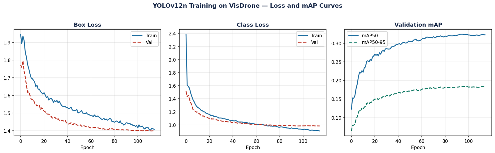
Figure 2 — Training curves for YOLOv12n on VisDrone at 640 resolution over 115 epochs. Box loss and class loss decrease steadily with validation closely tracking training, no overfitting. Validation mAP50 reaches 0.32 and mAP50-95 reaches 0.19 at convergence.
In our training run, box_loss dropped from 1.946 at epoch 1 to 1.41 at convergence. Class loss fell from 2.388 to 0.95. The model converged at epoch 115, reaching a validation mAP50 of 0.32 and mAP50-95 of 0.19.
One Mistake Per Stage That Will Kill Your Results
At the Annotation Stage
At the Dataset Preparation Stage
At the Training Stage
best.pt checkpoint based on validation mAP. Some users accidentally point their evaluation script at the training data rather than the validation data. Always verify which split your evaluation is running on before reporting any number.
At the Evaluation Stage
What Good Predictions Look Like — And What Failure Looks Like
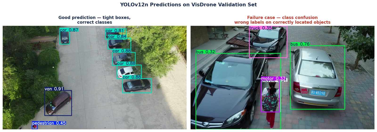
Figure 3 — YOLOv12n predictions on two VisDrone validation images. Left: a successful case, cars detected with high confidence (0.81–0.88), van at 0.91, and a small pedestrian correctly identified at 0.45. Right: a class confusion failure, vehicles are correctly located but misclassified as bus (0.32, 0.76) and truck (0.35).
from ultralytics import YOLO
import glob

model = YOLO(
    'visdrone_runs/yolo12n_baseline/weights/best.pt'
)

val_images = glob.glob(
    'visdrone/images/val/*.jpg')[:10]

for img_path in val_images:
    results = model.predict(
        img_path,
        conf=0.25,
        iou=0.45,
        save=True,
        project='predictions',
        name='val_sample'
    )
When you look at the prediction images, you are checking for three things:
- Are the boxes finding the right objects? Correct class labels on the majority of clearly visible objects means the model has learned the classes.
- Is class confusion occurring? On VisDrone specifically, visually similar classes, car, van, truck, bus, are commonly confused, especially when objects are small or partially visible.
- Are there obvious false positives? Background regions being detected as objects suggests the confidence threshold is too low, or the model has seen insufficient negative examples during training.
Where Most People Stop — And Why That Is the Problem
The steps above will get most people to a working baseline model. For many applications, that is enough.
But a baseline model on VisDrone is not a deployable model. A nano model at 640 resolution reaching mAP50 of 0.32 is a respectable starting point, it confirms your pipeline works and your data is correctly formatted. The harder work is understanding why the remaining 68% of objects are missed or misclassified, and which of those failures are addressable through better training strategy versus which are fundamental limitations of the model scale.
VisDrone has characteristics that a standard training run does not fully address: severe small-object density, large variations in altitude and scale, class imbalance between common classes like cars and rare ones like tricycles, and class confusion between visually similar vehicle types. That is exactly where the baseline ends and the real work begins.
Even after improving accuracy, deployment constraints still matter. Parameter count, latency, inference throughput, memory usage, and hardware limitations ultimately determine whether a detector remains useful outside controlled experimentation.
Continue Beyond the Baseline
This article focuses on building a reliable baseline detection pipeline. The next challenge is improving robustness, handling domain-specific failures, optimizing deployment constraints, and designing stronger experiments for real-world datasets.
📖 The Occulins detection book track expands these topics through structured workflows, deployment-oriented experimentation, and practical case studies.
Explore Detection BooksSelected implementations, supporting utilities, dataset templates, and companion resources related to this article are available through the Blog 2 Companion Resources page .
Companion Resources Included
- Dataset directory structure reference
- Label format verification utility
- Dataset YAML configuration example
- Baseline training workflow
- Inference and prediction utilities
- Evaluation checklist
Quick Reference
| Stage | Key Decision | Common Mistake |
|---|---|---|
| Dataset preparation | Verify label format and filename matching | Silently missing label files |
| Split strategy | Split at sequence level, not image level | Random split inflates validation mAP |
| Model scale | Start with nano, scale up after confirming setup | Training large model on misconfigured data |
| Image size | Use the 640 default — understand what it gives you | Changing image size before confirming data is correct |
| Pretrained weights | Always use COCO pretrained initialization | Training from scratch loses 5–15 mAP |
| Training monitoring | Watch box_loss, cls_loss, dfl_loss per epoch | Waiting until end to check predictions |
| Evaluation | Report both mAP50 and mAP50-95 | mAP50 alone overstates performance by up to 13 points |
Working on a detection project and running into challenges beyond what this post covers?
Feel free to reach out through occulinslab.com/contact