By Dr. Ali Khan | Occulins
August 15, 2026
Training a detection model is the part most tutorials cover in detail. Evaluating one properly is the part most tutorials rush through in two paragraphs.
This matters because evaluation is where model quality is actually measured. A model that looks good on one metric can look poor on another and the choice of metric determines what you optimise for, what failures you see, and whether your model is actually ready for deployment.
This post covers the evaluation pipeline for object detection from the ground up, IoU, precision, recall, the PR curve, AP, mAP, and the confidence threshold, using real results from a YOLOv12n model trained on VisDrone. Every figure in this post comes from an actual training run, not synthetic examples.
Step 1 — Intersection over Union
Before any metric can be computed, the evaluation pipeline needs to decide whether a predicted bounding box counts as a correct detection or not. This decision is made using Intersection over Union, IoU.
IoU measures the overlap between a predicted box and a ground truth box as a ratio of their intersection area to their union area:
IoU = Area of Intersection / Area of UnionAn IoU of 1.0 means the predicted box perfectly overlaps the ground truth. An IoU of 0.0 means no overlap at all. The IoU threshold determines the minimum overlap required for a prediction to count as a true positive.
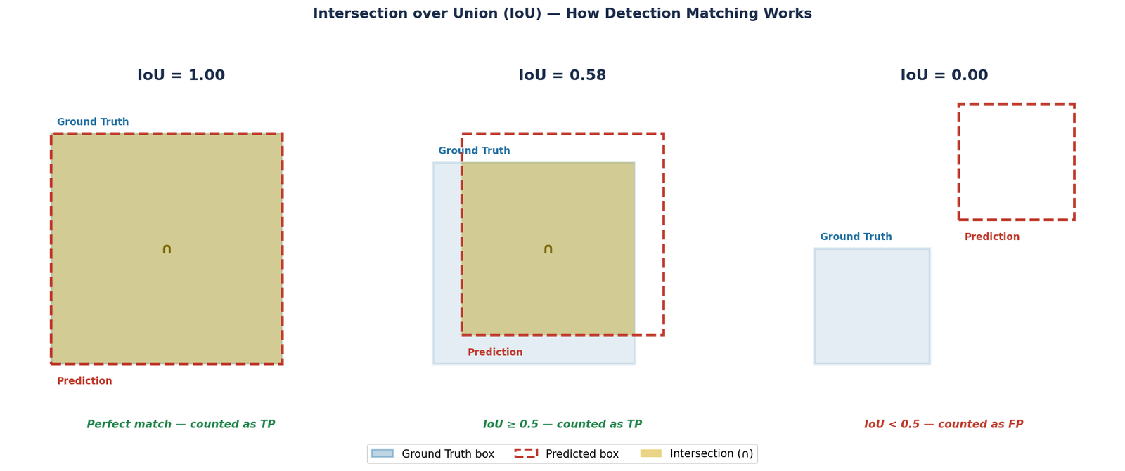
Figure 1 — Three IoU cases. Left: perfect overlap (IoU=1.00), counted as a true positive. Centre: partial overlap (IoU=0.58), above the standard 0.5 threshold and counted as a true positive. Right: no overlap (IoU=0.00), counted as a false positive regardless of confidence score.
The standard threshold for COCO-style evaluation is IoU=0.5, which is why mAP50 is the most commonly reported metric. A prediction must overlap the ground truth by at least 50% to be considered correct. This is a relatively lenient threshold, a box that overlaps by exactly 50% still has significant misalignment with the true object boundary.
Step 2 — Precision and Recall
Once IoU determines which predictions count as true positives, precision and recall measure two different aspects of detection quality.
Precision measures what fraction of your predictions were correct:
Precision = TP / (TP + FP)A model with high precision makes few false positive predictions. When it says an object is there, it is usually right. A model with low precision produces many false alarms.
Recall measures what fraction of actual objects were detected:
Recall = TP / (TP + FN)A model with high recall finds most of the objects in the scene. A model with low recall misses many objects even if the ones it does find are correct.
Precision and recall trade off against each other through the confidence threshold. Lowering the confidence threshold causes the model to report more detections, recall goes up because more true objects are found, but precision goes down because more false positives are also included. Raising the threshold has the opposite effect.
The Precision-Recall Curve
Rather than evaluating at a single threshold, the PR curve shows this trade-off across all possible confidence thresholds simultaneously. Each point on the curve represents a (precision, recall) pair at one threshold value.
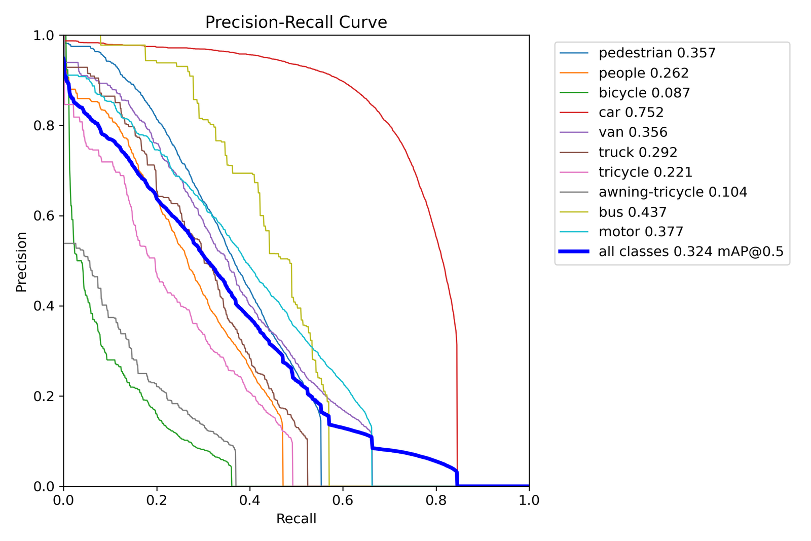
Figure 2 — Precision-Recall curves for YOLOv12n trained on VisDrone, evaluated at IoU=0.5. Each coloured line represents one class. Car (red, AP=0.752) achieves high precision across a wide recall range, the model finds cars reliably and confidently. Bicycle (green, AP=0.087) and awning-tricycle (grey, AP=0.104) collapse quickly, the model finds some but struggles to maintain precision as recall increases. The bold blue line shows the mean across all classes (mAP50=0.325).
The class performance gap visible in this figure tells the story of VisDrone's class imbalance. Car has 14,064 instances in the validation set, the model has seen enough examples to build reliable detectors. Bicycle has 1,287 instances and awning-tricycle has 532. With fewer examples and smaller visual signatures, these classes produce weaker PR curves and much lower AP scores.
Step 3 — Average Precision and mAP
The PR curve gives a complete picture of one class's detection performance, but comparing curves visually across classes is impractical. Average Precision summarises the entire PR curve as a single number, the area under the curve.
AP = area under the Precision-Recall curveUltralytics computes AP using the 101-point interpolation method, the precision is sampled at 101 evenly spaced recall values from 0 to 1, and the mean is taken. This is the COCO standard.
Mean Average Precision, mAP, is then the mean of AP across all classes:
mAP = mean(AP_class1, AP_class2, ..., AP_classN)mAP50 vs mAP50-95
mAP50 computes AP at a single IoU threshold of 0.5. mAP50-95 averages AP across ten IoU thresholds from 0.5 to 0.95 in steps of 0.05.
mAP50-95 is significantly harder to achieve than mAP50 because it requires the model to produce tight, precise bounding boxes, not just approximate locations. A box that overlaps by 52% counts at IoU=0.5 but fails at IoU=0.75.
For the YOLOv12n VisDrone model:
| Class | AP50 | Notes |
|---|---|---|
| pedestrian | 0.357 | Common but small — moderate performance |
| people | 0.262 | Similar to pedestrian, often confused |
| bicycle | 0.087 | Small, rare — weakest class |
| car | 0.752 | Most common, largest — strongest class |
| van | 0.356 | Confused with car and truck |
| truck | 0.292 | Confused with van and bus |
| tricycle | 0.221 | Small, visually similar to motor |
| awning-tricycle | 0.104 | Rare, small — second weakest |
| bus | 0.437 | Large, distinctive — good performance |
| motor | 0.377 | Common but small |
| all classes | 0.325 | mAP50 — mean across all classes |
Step 4 — The Confidence Threshold
mAP is computed at conf=0.001 — effectively no confidence filtering to capture the full PR curve. But at deployment, you need to choose a single confidence threshold that determines what the model actually reports.
The F1 score balances precision and recall into a single number:
F1 = 2 × (Precision × Recall) / (Precision + Recall)The F1-Confidence curve shows F1 at every possible confidence threshold. The peak of this curve is the optimal operating point, the threshold that best balances finding objects and avoiding false positives.
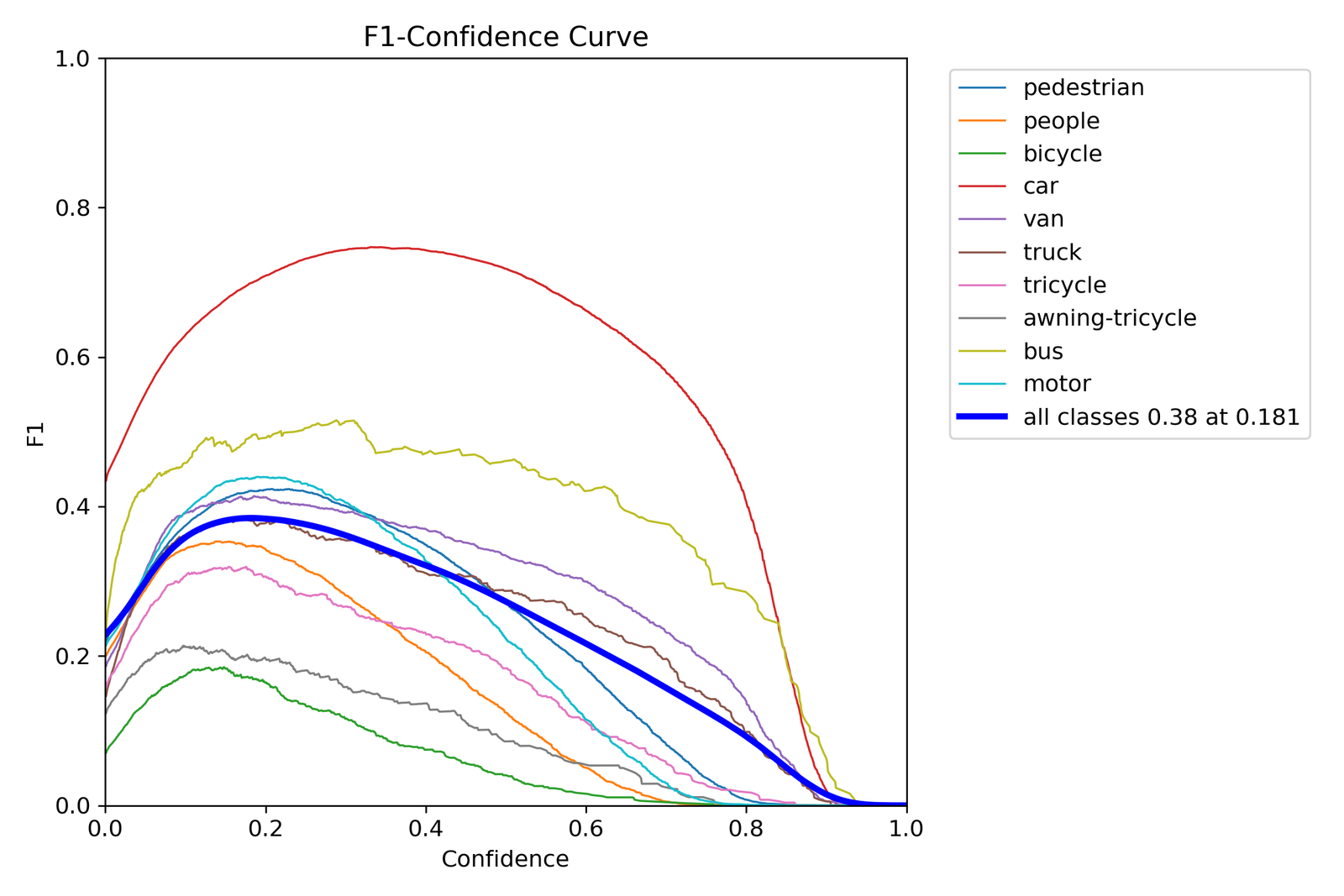
Figure 3 — F1-Confidence curves for YOLOv12n on VisDrone. The optimal confidence threshold across all classes is 0.181 (bold blue line, peak F1=0.38). Car (red) reaches F1=0.75 and remains high across a wide confidence range, the model is reliably confident on cars. Bicycle (green) and awning-tricycle (grey) peak below F1=0.20, these classes are detected so infrequently and at such variable confidence that no threshold produces good F1.
The optimal threshold of 0.181 is lower than the Ultralytics default of 0.25. This is typical for datasets with many small objects, the model produces correct detections at lower confidence scores for small targets, and using the default 0.25 threshold discards many of them.
The practical implication: if you use conf=0.25 for VisDrone inference, you are missing detections that the model found correctly but reported with confidence between 0.181 and 0.25. Running inference with conf=0.18 recovers these without substantially increasing false positives.
from ultralytics import YOLO

model = YOLO('yolo12n_baseline/weights/best.pt')

# Default threshold — misses low-confidence
# small object detections
results_default = model.predict(
    source='visdrone/images/val',
    conf=0.25,
    save=True,
    name='default_threshold'
)

# Optimal threshold from F1 curve
results_optimal = model.predict(
    source='visdrone/images/val',
    conf=0.18,
    save=True,
    name='optimal_threshold'
)
Step 5 — The Confusion Matrix
mAP and the PR curve tell you how well the model detects objects overall. The confusion matrix tells you specifically which classes are being confused with which other classes, a different and equally important question.
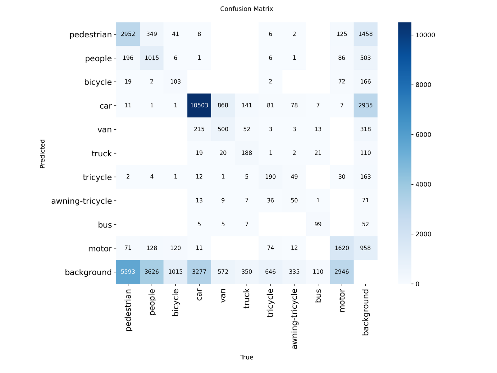
Figure 4 — Confusion matrix for YOLOv12n on the VisDrone validation set. Rows are predicted classes, columns are true classes. The diagonal represents correct detections. The rightmost column (background) shows objects that were missed entirely, not detected at all. The bottom row (background) shows false positives, detections where no ground truth object existed. Car is the best-performing class with 10,503 correct detections. The large background column for pedestrian (1,458 missed) and motor (2,946 missed) confirms that small object classes have high miss rates.
Three patterns are immediately visible from the confusion matrix:
Vehicle class confusion. Cars are frequently predicted as vans (868) and vans predicted as cars (215). Trucks are confused with vans in both directions. This is expected — from aerial altitude these vehicle types have similar rectangular top-down profiles and similar sizes.
Large background column. Every class has a substantial number of ground truth objects that were missed entirely, predicted as background. Pedestrian misses 1,458, motor misses 2,946, car misses 2,935. These represent the fundamental recall limitation of the model.
Large background row. The model also produces false positives, 5,593 for pedestrian alone. These are detections where the model predicted a pedestrian but no ground truth object existed at that location. High false positive rates in a class suggest the model is finding visual patterns that look like the class but are not.
Putting It Together — What to Report
A complete evaluation of a detection model should include all of the following:
| Metric | What it tells you | How to get it |
|---|---|---|
| mAP50 | Overall detection quality at lenient IoU | model.val() |
| mAP50-95 | Overall localisation quality | model.val() |
| Per-class AP50 | Which classes are detected well vs poorly | PR curve legend |
| Optimal confidence | Best operating threshold for deployment | F1 curve peak |
| Confusion matrix | Which classes are confused with each other | Saved during validation |
| False negative rate | What fraction of objects are missed | Background column of confusion matrix |
For the YOLOv12n VisDrone baseline the complete picture is: mAP50=0.325, mAP50-95=0.185, optimal confidence=0.181, car is the strongest class at AP50=0.752, bicycle and awning-tricycle are the weakest at 0.087 and 0.104, and the model misses a substantial fraction of small objects in every class. This is a complete and honest characterization, not just a single number.
Selected implementations, supporting utilities, and companion resources related to this article are available through the Blog 7 Companion Resources page .
Companion Resources Included
- IoU computation
Working on an object detection project and unsure how to interpret your evaluation results?
Reach out through
Occulins Contact
for deployment-aware computer vision research and engineering support.