By Dr. Ali Khan | Occulins
September 4, 2026
Getting a model to train successfully is the part tutorials teach well. Getting that model to work reliably in a real system is the part they consistently skip.
The gap between a working notebook and a working deployment is wider than most people expect when they first encounter it. It is not primarily a technical gap, the tools exist, the documentation is available, and the steps are learnable. It is a thinking gap. The questions you need to answer before deploying a model are fundamentally different from the questions you asked while training it, and nobody explicitly tells you that the questions have changed.
This post covers what that gap actually looks like, the questions that determine whether your deployment succeeds, and where detection and segmentation problems differ in ways that matter at the system level. The benchmark numbers throughout come from running YOLOv12n and YOLOv12s, the same models trained on VisDrone throughout this series, through TensorRT on an RTX 4090 Laptop GPU.
The Environment Has Changed — and It Changes Everything
During training, your environment is optimised for model development. You have a powerful GPU, unlimited time per inference, Python with all its dependencies, and a dataset that is already cleaned and formatted. None of these will be true at deployment.
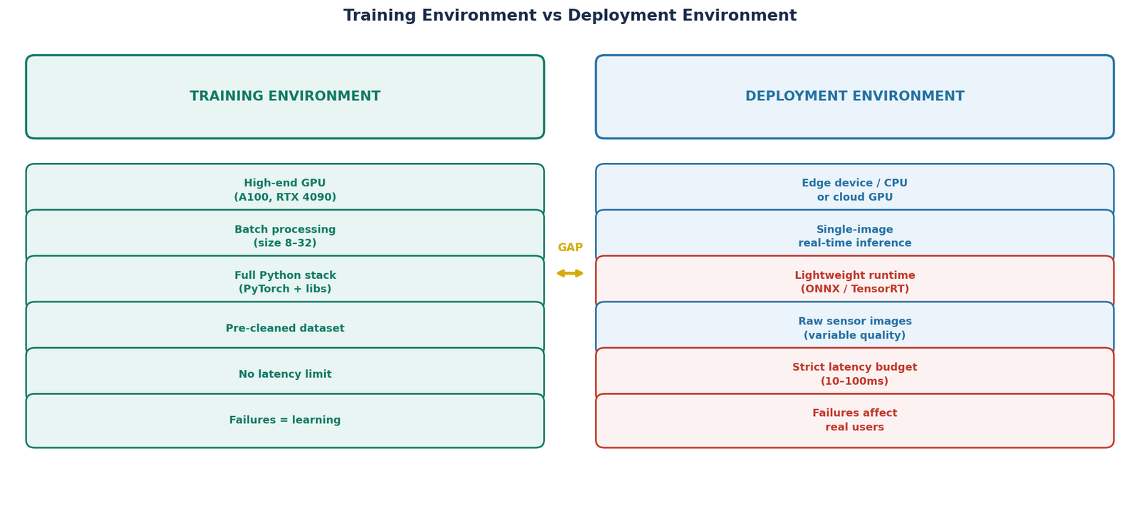
Figure 1 — Training environment versus deployment environment. The three items highlighted in red,lightweight runtime, strict latency budget, and failures affecting real users, are the constraints that most commonly cause problems in deployment. None of them exist during training.
Training Environment
- High-end GPU (A100, RTX 4090)
- Batch size 8–32 for throughput
- Python + PyTorch full stack
- Pre-cleaned, pre-resized images
- No latency requirement
- Failures are learning opportunities
- You control the hardware
Deployment Environment
- Edge device, CPU, or shared cloud GPU
- Batch size 1 for real-time processing
- Runtime must be lightweight
- Raw images from camera or sensor
- Strict latency requirement
- Failures affect real users
- Hardware is fixed
The most consequential change is the shift from batch inference to single-image inference. During training, you measure throughput which tells you how many images per second the GPU can process. At deployment, you measure latency that determines how long a single image takes from input to output. These are not the same thing and they do not optimize for the same conditions.
A model that achieves 200 images per second in batch processing may take 80 milliseconds for a single image on the same hardware. If your application requires 30fps real-time processing, 80ms per image is not fast enough and no amount of batch optimization changes that, because you only have one image to process at a time.
Real Latency Numbers — YOLOv12 on RTX 4090
The numbers below come from running YOLOv12n and YOLOv12s through TensorRT on an RTX 4090 Laptop GPU. Each configuration was benchmarked with 50 warmup iterations followed by 200 timed iterations at single-image inference, 640×640. The inference thresholds used were conf=0.25 (Ultralytics default inference confidence) and iou=0.5 (the NMS sweet spot identified for VisDrone in Blog 6). These are real deployment thresholds — not the evaluation protocol values of conf=0.001 used for mAP computation — so the latency numbers reflect actual production behaviour rather than benchmark-only conditions.
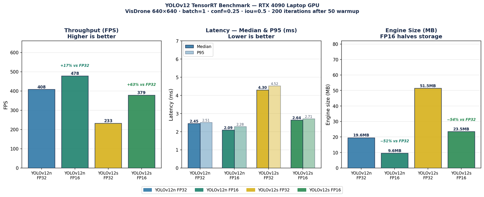
Figure 2 — Real TensorRT benchmark results on RTX 4090 Laptop GPU (conf=0.25, iou=0.5, 200 iterations after 50 warmup). Left: throughput — FP16 gives +17% speedup on nano and +63% on small. Centre: latency median and P95 — all four configurations are well below 5ms. Right: engine size — FP16 halves storage in both cases. All results from real inference runs on VisDrone-trained checkpoints.
| Model | Precision | FPS | Median (ms) | P95 (ms) | Engine (MB) | mAP50 |
|---|---|---|---|---|---|---|
| YOLOv12n | FP32 | 408 | 2.45 | 2.51 | 19.6 | 0.325 |
| YOLOv12n | FP16 | 479 | 2.09 | 2.28 | 9.6 | 0.325 |
| YOLOv12s | FP32 | 233 | 4.30 | 4.52 | 51.5 | 0.419 |
| YOLOv12s | FP16 | 379 | 2.64 | 2.71 | 23.5 | 0.419 |
Three findings stand out. First, FP16 is the correct default for NVIDIA deployment which gives 17% speedup on nano and 63% on small with identical mAP50, and halves engine size in both cases. Second, even the slowest configuration (YOLOv12s FP32 at 4.3ms) is fast enough for real-time video at any standard frame rate. Third, the P95 latency is close to the median in all configurations where YOLOv12n FP16 has median 2.09ms and P95 2.28ms, a gap of just 0.19ms, indicating a stable, consistent engine with no significant tail latency spikes.
The accuracy-latency trade-off is also clear. YOLOv12s FP16 achieves mAP50=0.419 at 2.64ms, 29% better accuracy than nano at only 26% more latency. For applications where latency budget is not the binding constraint, the small model is the better deployment choice.
The Latency Budget Question
Your latency budget is determined by your application, not by your model. Some common reference points:
| Application | Latency budget | Frame rate implied |
|---|---|---|
| Real-time video surveillance | 33ms per frame | 30 fps |
| Drone autonomous navigation | 50–100ms | 10–20 fps |
| Medical image analysis (non-real-time) | 500ms–5s | Batch, not real-time |
| Industrial inspection on conveyor | 10–50ms | 20–100 fps |
| Clinical decision support (offline) | No strict constraint | Not applicable |
Know your latency budget before choosing your model. Measure actual latency on your actual deployment hardware, not on your training GPU. The two can differ by a factor of 5 to 20 depending on the hardware combination.
Model Format and Runtime
A PyTorch model saved as a .pt checkpoint file requires the full PyTorch stack to run. In many deployment environments the full PyTorch stack is either unavailable, too slow, or consuming memory that your application needs for other purposes. Two tools address this.
ONNX (Open Neural Network Exchange) is an open format for representing trained models that is independent of the training framework. Exporting to ONNX allows a model trained in PyTorch to be run with ONNX Runtime, a lightweight inference engine available on a much wider range of hardware than PyTorch and typically 20 to 40% faster for single-image inference.
from ultralytics import YOLO

model = YOLO('best.pt')

# Export to ONNX — cross-platform deployment
model.export(
    format='onnx',
    imgsz=640,
    batch=1,
    opset=12
)
TensorRT is NVIDIA's inference optimisation library. It compiles a model into an optimised engine for the target GPU, applying layer fusion, precision reduction, and kernel selection to minimise latency. TensorRT engines are 2 to 4 times faster than PyTorch on NVIDIA hardware.
from ultralytics import YOLO

model = YOLO('best.pt')

# Export to TensorRT FP16 — fastest on NVIDIA
model.export(
    format='engine',
    imgsz=640,
    batch=1,
    half=True,      # FP16 — faster, same mAP
    workspace=4.0,  # GB for optimisation
    device=0
)

# Load and run the engine
# conf=0.25 and iou=0.5 are deployment thresholds
# NOT the conf=0.001 used for mAP evaluation
engine = YOLO('best.engine', task='detect')
results = engine.predict(
    source='image.jpg',
    conf=0.25,   # deployment confidence threshold
    iou=0.5      # NMS sweet spot for VisDrone (Blog 6)
)conf=0.25 and iou=0.5 — real deployment values. The mAP evaluation in earlier blogs used conf=0.001 and iou=0.7. Never use conf=0.001 in production — it generates far more candidate predictions before NMS, inflates postprocessing time, and does not represent real deployment behaviour.
For most projects the practical path is: train in PyTorch → validate in PyTorch → export to ONNX for cross-platform deployment → export to TensorRT if you are on NVIDIA hardware and need maximum speed.
Five Questions You Must Answer Before Deploying
Not your training GPU — your deployment hardware. This determines which model format to use, what the achievable latency actually is, and whether FP16 or INT8 quantisation is an option. If you do not know the deployment hardware, you cannot make any of the other decisions correctly.
Define it precisely — in milliseconds per image — before evaluating any model. A model that meets your accuracy requirement but not your latency requirement is not deployable, regardless of how good the mAP is. From the benchmark results above: YOLOv12n FP16 at 2.09ms and YOLOv12s FP16 at 2.64ms (both at conf=0.25, iou=0.5) comfortably fit any real-time application on an RTX 4090. On a Jetson Orin or a CPU, these numbers will be substantially different — always measure on the target hardware.
Note: the benchmark used conf=0.25 and iou=0.5 — real inference thresholds, not the conf=0.001 used for mAP evaluation. Latency numbers from evaluation-mode inference would be higher due to the larger number of predictions processed before NMS.
During training, images were pre-loaded and pre-processed. At deployment, images arrive from a camera, a sensor, a file upload, or a network stream — in different formats, at different resolutions, with different colour profiles. The pre-processing pipeline that converts incoming images to the format your model expects is a real engineering problem that is completely absent from training notebooks.
During training, a wrong prediction is a loss value. At deployment, a wrong prediction has consequences that depend on the application. A missed vehicle detection in a surveillance system is logged. A missed lesion in a clinical screening system may affect patient care. Define what happens on failure before you deploy, and design the system to handle it — not just to produce outputs.
Models deployed in the real world encounter distribution shift — images from cameras with different characteristics, different lighting conditions, different seasons. Without monitoring, you will not know when your model's real-world performance has drifted from its validation metrics. Define a monitoring strategy before deployment, not after you notice a problem.
Where Detection and Segmentation Differ at Deployment
The five questions above apply equally to both tasks. But detection and segmentation have different characteristics at the system level that affect deployment decisions.
Output Size and Post-Processing
A detection model produces a list of bounding boxes, typically tens to hundreds of boxes per image after NMS. This is a compact output that is easy to pass to downstream systems, store, or transmit.
A segmentation model produces a dense output — a class label for every pixel in the image. At 1920×1080 resolution with 10 classes, the raw output is a large float32 tensor before any compression. Storing, transmitting, or processing this output requires explicit decisions about compression, downsampling, or sparse representation that detection deployments do not require.
Latency Characteristics
Detection models spend most inference time in the backbone and neck. Post-processing (NMS) adds a small fixed cost. Segmentation models spend inference time in both the encoder and the decoder — the decoder adds substantial computation with no equivalent in detection. At the same backbone, a segmentation model is typically 30 to 60% slower than a detection model due to decoder cost.
Threshold Sensitivity
Detection models have a confidence threshold — objects below it are discarded. For VisDrone we found conf=0.25 with iou=0.5 to be the right deployment operating point (Blog 6). Segmentation models produce a continuous probability map and the threshold that converts this to a binary mask is a deployment parameter that directly affects the precision-recall operating point. This threshold should be chosen on your deployment data, not on your training validation set.
What Tutorials Consistently Skip
Tutorials show you how to get a model working in a clean, controlled environment. They consistently omit four things that determine whether that model works in a real environment.
Pre-processing pipelines. The model expects images at a specific size, in a specific colour format, normalised in a specific way. In deployment, images arrive in whatever format the camera or sensor produces. Writing a robust pre-processing pipeline that handles edge cases, rotated images, corrupted files, unexpected resolutions, colour space mismatches — is unglamorous work that tutorials skip and real deployments require.
Error handling. What should the system do when inference takes three times longer than expected? When the model produces no detections on a frame where there should be objects? When the input image is corrupted? These failure modes need explicit handling in production systems. They are completely absent from tutorial notebooks.
Model versioning. When you improve your model and want to deploy an updated version, you need a strategy for switching versions without disrupting the running system. This requires thinking about model storage, version identifiers, and rollback capability before you have a second version to deploy, not after.
Performance measurement in production. Latency measured on a benchmark GPU tells you the theoretical minimum. The numbers in this post, 2.09ms for YOLOv12n FP16, 2.64ms for YOLOv12s FP16, both at conf=0.25 and iou=0.5, are model-only inference times. Latency in production also includes network transfer time, pre-processing time, queue waiting time, and post-processing time. The number that matters is end-to-end latency from input to output in the real system. Measure the former, not the latter.
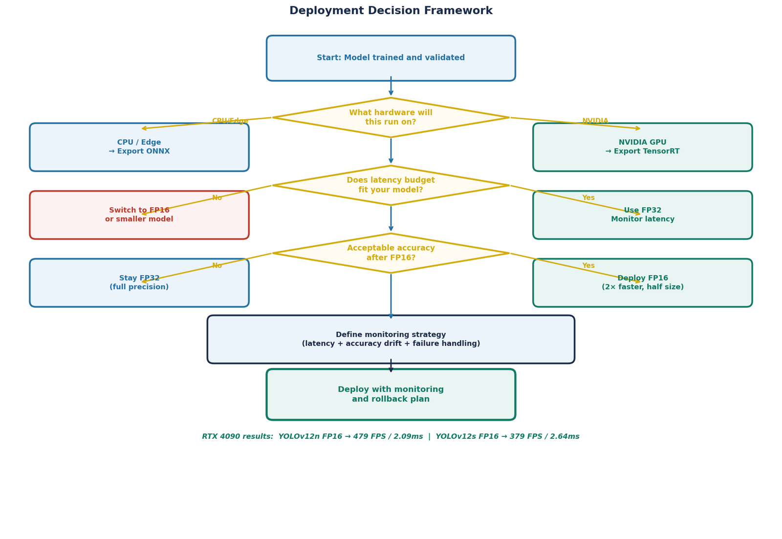
Figure 3 — Deployment decision framework. Starting from hardware, NVIDIA leads to TensorRT, CPU or edge leads to ONNX. The latency branch determines whether FP32 is sufficient or FP16 is needed. The precision validation branch confirms FP16 accuracy before committing. Real benchmark results annotated at the bottom: YOLOv12n FP16 → 479 FPS / 2.09ms, YOLOv12s FP16 → 379 FPS / 2.64ms, both measured at conf=0.25, iou=0.5.
The Decisions That Require Domain Expertise
The technical steps of deployment, exporting to ONNX, optimising with TensorRT, writing a pre-processing pipeline, are learnable from documentation. The decisions that determine whether the deployment succeeds are harder to learn from documentation because they depend on context that documentation cannot know.
What accuracy-latency trade-off is acceptable for your specific application? Which failure mode matters more, a false positive or a missed detection, and how should the model's operating threshold reflect that? How will you validate that the deployed model's real-world performance matches its validation metrics? When performance degrades, how will you know whether to retrain, to adjust thresholds, or to investigate the data pipeline?
These questions do not have universal answers. They depend on the specific application, the specific hardware, the specific data distribution, and the specific consequences of failure. Answering them correctly requires experience with similar deployments and judgment about which trade-offs matter most for the problem at hand.
That is the space where the gap between a model that technically works and one that works reliably in production actually lives.
Selected implementations, supporting utilities, and companion resources related to this article are available through the Blog 9 Companion Resources page .
Companion Resources Included
- TensorRT engine export function
- Benchmark timing function
- Benchmark configuration reference
Working on deploying a detection or segmentation model and running into decisions that do not have clear answers?
Reach out through
Occulins Contact
for deployment-aware computer vision research and engineering support.