By Dr. Ali Khan | Occulins
September 10, 2026
There is a specific kind of frustration that comes after a detection project has technically succeeded. The model is trained. The mAP looks competitive. The validation predictions pass a quick visual check. Then you test it in the actual deployment environment and the failures start appearing such as objects missed entirely, wrong classes predicted with high confidence, performance that bears no resemblance to the validation numbers.
This is not a rare edge case. It happens in the majority of detection projects at some point, and it has happened in projects I have worked on. The pattern is consistent enough that I can describe it precisely: the model learned to perform well on the evaluation setup rather than on the underlying task. The evaluation setup and the underlying task felt identical during development. They were not.
This post covers four specific mechanisms that produce this failure. Each one is subtle enough to pass through a standard training and evaluation workflow without being detected. Each one has a specific signature that reveals it if you know what to look for.
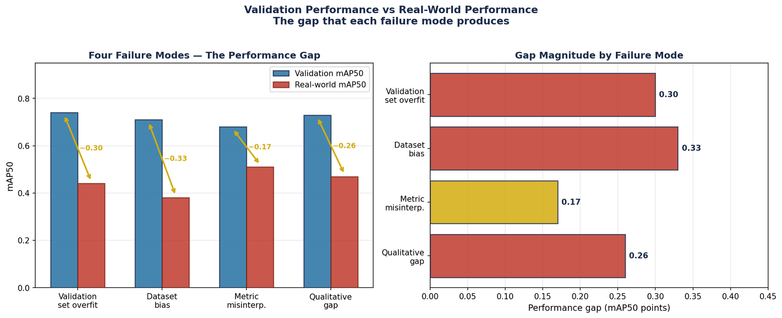
Figure 1 — The performance gap between validation metrics and real-world deployment for each of the four failure modes covered in this post. Dataset bias produces the largest gap at 0.33 mAP50 points showing a model that appears strong on validation is barely functional on deployment data. Note: figures are illustrative. The pattern is consistent across projects; the specific values vary.
This is not the classic overfitting that training loss curves reveal where training loss decreases and validation loss rises. That version is easy to detect and easy to fix with early stopping. The version that causes real-world failures is subtler and more insidious.
It happens when the validation set is not genuinely independent of the training data. The model has not memorised the validation images it has learned features that are specific to the data source rather than specific to the objects of interest. On validation images from the same source, those features are reliable predictors. On images from any other source, they are noise.
The Mechanism
Consider a drone detection project where training and validation images all come from the same fleet of drones operated in the same geographic area during the same season. The model achieves strong mAP on validation. Then you deploy it on footage from a drone with a different camera, or from a different location, or three months later when vegetation has changed. Performance collapses.
The model did not learn "what a vehicle looks like from above." It learned "what a vehicle looks like from above in footage from this specific fleet, in this specific location, in this specific season." The validation set, drawn from the same fleet and location, could not reveal this limitation because it shared all the same idiosyncrasies.
What It Looks Like
Validation mAP is strong typically within a few points of the training mAP. There is no obvious overfitting signal in the loss curves. The model passes quick visual inspection on validation images. Then it encounters images from a slightly different camera, lighting condition, altitude, or geographic area and fails significantly more than the validation numbers would predict.
Dataset bias occurs when the model learns a feature of the dataset that correlates with the target class in the training data but does not represent the target class itself. The model is doing exactly what supervised learning is supposed to do that is finding the strongest signal for the class, but the strongest signal is an artefact of how the dataset was collected, not a genuine property of the objects.

Figure 2 — Background correlation bias. Vehicles on tarmac (training data, left) are all detected with high confidence. The same vehicles on grass (deployment, right) produce four misses and one weak detection at confidence 0.31. The model learned the background, not the vehicle.
Background Correlation
The most common form of dataset bias in detection is background correlation where objects of a particular class appear disproportionately against certain backgrounds in the training data. A vehicle detector trained on urban aerial imagery may have learned features of tarmac roads as strongly as features of vehicles. In deployment, when vehicles appear in car parks, on gravel, or on unpaved roads, the model's confidence drops because the road texture it learned to associate with vehicles is absent.
This is not a failure of the model, it is a failure of the dataset. The model found the optimal solution given the data it was trained on. The problem is that "optimal for this data" was not the same as "correct for this task."
Acquisition Protocol Correlation
In medical imaging, a particularly damaging form of dataset bias is acquisition protocol correlation. When all images of a rare condition in a training dataset happen to come from one scanner or one institution, the model may learn features of that scanner's image characteristics rather than features of the condition itself. On images from other scanners, the apparent prevalence of the condition in the model's predictions drops dramatically.
I have seen this pattern in skin lesion detection where images of one class were collected at a different dermoscope magnification than images of another class. The model learned the magnification as a class indicator. The evaluation within the dataset showed high accuracy. The evaluation across magnifications revealed the bias.
Temporal Correlation in Video Sources
When training data comes from video sequences and images are split randomly at the image level, consecutive frames from the same scene appear in both training and validation sets. The model effectively memorises scene-specific features, specific road markings, specific building configurations, specific tree placements, that are present in training frames and identical in nearby validation frames. This produces validation mAP that reflects scene memorisation rather than generalisation.
This failure mode does not affect how the model performs. It affects how you understand how the model performs. The model may be doing exactly what the metric says and the metric may not be measuring what you think it is measuring, or what your application actually requires.
mAP50 as a Proxy for mAP50-95
An earlier post in this series covered the difference between mAP50 and mAP50-95 in technical detail. The practical consequence for real-world deployments is worth restating directly: a model with mAP50 of 0.72 and mAP50-95 of 0.42 is a model where the majority of correct detections overlap the ground truth by 50 to 70%, correct enough to count at threshold 0.5, not precise enough to count at threshold 0.75 or above.
For applications where the bounding box is used downstream, feeding a tracking system, guiding a measurement, triggering a cropped region for classification, imprecise boxes cause real failures that mAP50 alone cannot reveal. The model looked good on the metric you reported. It failed on the task the metric was not measuring.
Mean AP Hiding Per-Class Failure
A detection model trained on ten classes with mAP50 of 0.68 may be achieving 0.85 on the seven common classes and 0.30 on the three rare ones. Reporting the mean presents a number that is not representative of performance on any individual class. If the rare classes are the ones that matter for your application and in safety-critical contexts they often are, because rare events are typically the dangerous ones, the mean metric is actively misleading.
Benchmark Performance as Deployment Performance
Benchmark datasets are constructed to be fair and reproducible. They are not constructed to represent your specific deployment environment. A model that achieves competitive mAP on VisDrone was evaluated on VisDrone's specific altitude range, camera specifications, geographic locations, and annotation standards. It was not evaluated on your drone, your camera, your location, or your annotation standards.
Benchmark performance is a useful signal about a model's general capability. It is not a prediction of your deployment performance. The only number that tells you about deployment performance is measurement on your deployment data.
This is the most subtle failure mode and the one that is hardest to systematise a fix for. The model achieves acceptable quantitative metrics, mAP, per-class AP, precision, recall — and produces predictions that a domain expert, looking at them directly, would immediately identify as wrong in a way the metrics cannot capture.
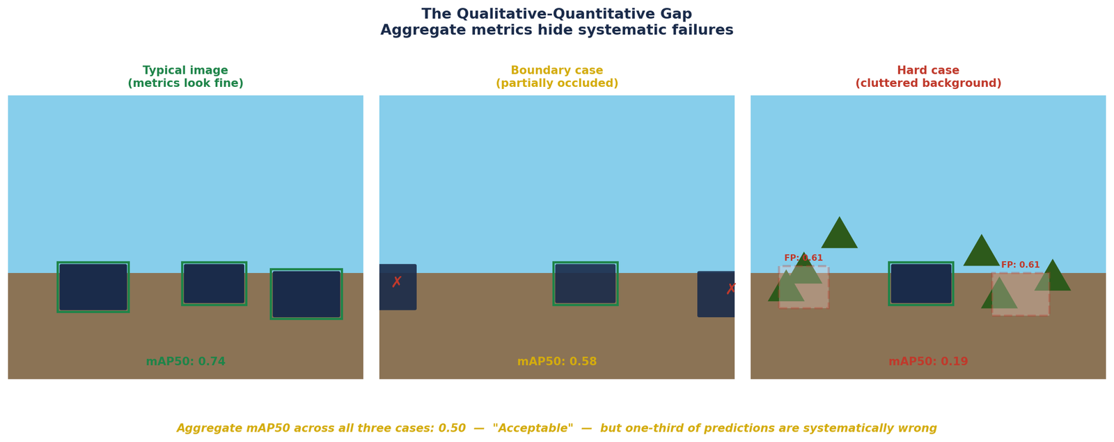
Figure 3 — The qualitative-quantitative gap. Typical images produce clean detections (mAP50: 0.74). Boundary cases produce systematic misses (mAP50: 0.58). Cluttered backgrounds produce false positives a domain expert would immediately reject (mAP50: 0.19). Aggregate mAP50 across all three: 0.50 — acceptable on paper, systematically wrong in one third of cases.
What the Gap Looks Like
The qualitative-quantitative gap appears in specific forms depending on the task.
In aerial detection, it often appears as a pattern of missed detections that are spatially correlated, the model consistently misses objects in the top-left or bottom-right corners of images, or consistently fails near image boundaries. The mAP averages over all positions and the positional bias is invisible in the aggregate. A domain expert looking at a grid of predictions sees the pattern in minutes.
In medical image detection, it often appears as false positives that are clinically implausible, the model detects objects in anatomical regions where the target class cannot exist, or produces detections with spatial extent that no expert would accept as plausible. The mAP counts these as false positives and penalises them in the precision calculation, but if they are rare enough relative to true positives, the aggregate metric remains acceptable while the outputs are clinically unacceptable.
In industrial inspection, it often appears as inconsistent confidence scores, the model produces high-confidence correct detections on easy examples and low-confidence incorrect detections on hard ones, but the aggregate mAP averages these together. A practitioner deploying at a fixed confidence threshold discovers that the model's performance degrades severely at the threshold they need to operate at.
Why Metrics Cannot Fully Capture Expert Judgment
Metrics measure what they are defined to measure. mAP measures detection precision and recall averaged across IoU thresholds and classes. It does not measure whether the predicted boxes are physically plausible, whether the detection pattern makes spatial sense, whether the confidence calibration is reliable, or whether the failure modes are acceptable for the application.
Expert judgment captures all of these things simultaneously and implicitly. An experienced practitioner looking at predictions brings domain knowledge that no scalar metric encodes knowledge about what a correct detection should look like, where false positives are acceptable and where they are not, and what failure patterns indicate fundamental model problems versus incidental noise.
The Common Thread
All four failure modes share the same underlying structure: the evaluation setup does not fully represent the deployment environment, and the gap between the two is invisible during development.
Validation set overfitting occurs when the validation set is too similar to the training data. Dataset bias occurs when the training data is too narrow. Metric misinterpretation occurs when the reported metric does not capture the application requirement. The qualitative-quantitative gap occurs when scalar metrics do not capture domain-relevant failure modes.
In each case, the model is doing its job correctly which is finding the optimal solution given the data and the objective it was trained on. The failure is in the assumptions made about what "optimal given this data and objective" means for the real deployment task.
Catching These Failures Before Deployment
| Failure Mode | Detection Method | When to Check |
|---|---|---|
| Validation set overfitting | Evaluate on independent test data from different source | Before declaring model ready |
| Dataset bias | Stratify evaluation by acquisition source, location, time | During dataset analysis and after training |
| Metric misinterpretation | Report per-class AP and mAP50-95 alongside mAP50 | Every evaluation run |
| Qualitative-quantitative gap | Expert review of random prediction sample | Before finalising evaluation and before deployment |
None of these checks are technically demanding. They do not require new tools or new infrastructure. They require the discipline to look at your model's behaviour in ways that go beyond the default evaluation output and the experience to know what you are looking for when you do.
The practitioners who catch these failures before deployment are not the ones with the most sophisticated evaluation pipelines. They are the ones who have been surprised by the gap between metrics and reality enough times to stop trusting metrics uncritically.
Selected implementations, supporting utilities, and companion resources related to this article are available through the Blog 10 Companion Resources page .
Companion Resources Included
- Failure mode detection checklist
- Symptom & catch reference
Working on a detection project where the metrics look right but something feels off about the real-world behaviour?
Feel free to reach out through
Occulins Contact