Common Mistakes in Object Detection Training
That Kill Performance
Object detection training failures share an uncomfortable characteristic: they are often invisible until you look in the right place.
A model can train for a hundred epochs, produce a respectable mAP number, and still be fundamentally broken, predicting the wrong classes, failing on the objects that matter most, or performing well only because the validation set leaked into training. The loss curves look fine. The metrics look acceptable. The predictions on casual inspection look plausible.
After years of working on detection problems across aerial imagery, medical imaging, and industrial inspection, I have seen the same mistakes appear repeatedly, not because the people making them are careless, but because the mistakes are genuinely subtle and the feedback signals that would reveal them are easy to overlook.
This post covers four of them. Each one has a specific symptom pattern that tells you it is present, and a specific fix that resolves it. None of them require changing your architecture or your hardware. All of them require paying closer attention to things you may currently be skipping.
This is the most common root cause of poor detection performance, and the one most rarely investigated because it requires looking at data rather than adjusting training parameters.
Annotation errors come in several forms, and they have different effects on training. Understanding which type you have determines what to do about it.
Tight vs Loose Bounding Boxes
Different annotators, or even the same annotator on different days, draw bounding boxes with different tightness. One person draws the box flush to the visible object edges. Another adds a few pixels of margin. A third includes part of the background context.
When a model is trained on this mixed data, it learns an inconsistent definition of where an object ends and background begins. During inference, predicted boxes are evaluated against ground truth boxes using IoU. If your ground truth boxes are inconsistently sized, your IoU measurements are measuring annotator inconsistency as much as model performance.
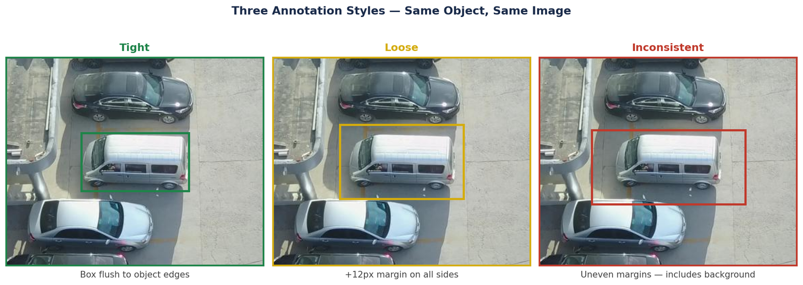
Figure 1 — Three annotation styles on the same object: tight (flush to visible edges), loose (2–5px margin), and inconsistent (partial background included). A training set mixing all three styles produces a model that learns no consistent boundary definition.
Inconsistent Class Definitions
This is harder to detect and more damaging than box tightness variation. It happens when the same visual object is labelled differently depending on context, annotator, or a class definition that was never written down precisely.
Common examples: a partially occluded car labelled as "car" in one image and ignored in another. A person on a bicycle labelled as "person" in some images and "cyclist" in others when cyclist is not a defined class. A van labelled as "car" by one annotator and "truck" by another.
The symptom in training is a class loss that decreases slowly or plateaus early, and a confusion matrix where two specific classes consistently swap with each other. If you see that pattern, look at the annotations for those two classes directly.
The Silent Problem: Missing Labels
In YOLO format, an image with no objects should have an empty label file. An image with objects but a missing label file is treated as a negative example — the model is taught that the objects in that image are background. This is one of the most damaging annotation errors because it actively teaches the model wrong information, not just inconsistent information.
Verify this before training:
import os

img_dir   = 'dataset/images/train'
label_dir = 'dataset/labels/train'

missing = []
for img_file in os.listdir(img_dir):
    stem       = os.path.splitext(img_file)[0]
    label_file = os.path.join(label_dir, stem + '.txt')
    if not os.path.exists(label_file):
        missing.append(img_file)

print(f"Images with no label file: {len(missing)}")
for f in missing[:10]:
    print(f"  {f}")
If this returns more than zero for a dataset that should have objects in every image, the missing label files are training your model to ignore those objects.
Data augmentation is universally recommended, and for good reason, it is one of the most effective tools for improving generalization on limited datasets. But augmentation is not a dial you turn up for better performance. The wrong augmentation strategy can actively damage your model, and the damage is difficult to diagnose because the training metrics often look fine while it is happening.
Augmentation That Destroys Small Objects
The most common augmentation mistake in detection is applying aggressive random cropping or zooming-out on datasets where objects are small relative to the image. When you randomly crop 40% of a 640×640 image, a pedestrian that was 20 pixels tall may disappear entirely, but its label file still says a pedestrian is present. The model is being trained on images where the labelled object is no longer visible.
For aerial datasets with small objects, the safe augmentation operations are flipping, rotation, and mild color jitter. Heavy cropping, large-scale mosaic augmentation with significant zoom-out, and perspective transforms that shrink objects further are all candidates for removal.
Color Augmentation on Domain-Specific Imagery
Aggressive color jitter is appropriate for natural photography where color balance varies widely between cameras and lighting conditions. It is not appropriate for datasets acquired under controlled conditions, certain medical imaging formats, thermal imagery, or nighttime surveillance footage where color characteristics are fixed by the acquisition protocol.
If your deployment images will always look roughly the same in terms of color and exposure, training on aggressively color-jittered images teaches the model to be robust to variation it will never encounter, while reducing its precision on the actual color characteristics of your domain.
Mosaic Augmentation and Dense Small Objects
YOLO's mosaic augmentation combines four images into one training sample. For most datasets this improves performance by exposing the model to more objects per forward pass. For datasets with very dense small objects, aerial imagery, crowd detection, microscopy, mosaic can produce images where object density exceeds anything in the real deployment distribution. The model learns to expect densities it will never see, which affects both detection thresholds and confidence calibration.
This mistake does not affect how your model trains. It affects whether you know what your model can actually do. Reporting the wrong metric, or computing the right metric on the wrong data, produces numbers that look good while hiding real failures.
mAP50 vs mAP50-95: A Gap That Changes Everything
mAP50 evaluates detection at a single IoU threshold of 0.5. A predicted box that overlaps the ground truth by 50% counts as a correct detection. This is a lenient standard, a box that covers the correct general region but is significantly larger or smaller than the actual object still passes.
mAP50-95 averages detection performance across IoU thresholds from 0.5 to 0.95 in steps of 0.05. At IoU 0.75, a predicted box needs to overlap 75% with the ground truth to count. At IoU 0.95, the box needs to be almost pixel-perfect.
For applications where precise bounding box location matters, measuring object size, feeding detections into a tracking system, or using boxes to guide downstream processing — mAP50-95 is the metric that tells you whether your model is accurate enough. mAP50 can look 15 to 25 points higher than mAP50-95 on the same model.
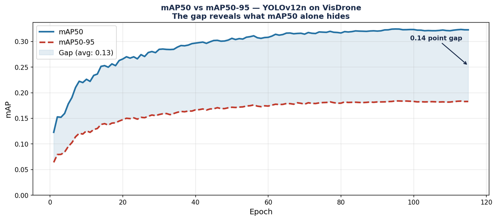
Figure 2 — mAP50 vs mAP50-95 across training epochs for YOLOv12n on VisDrone. mAP50 reaches 0.325 while mAP50-95 plateaus at 0.185, a gap that reflects the model's ability to find objects in the right location but not localise them precisely. The shaded region between the two curves is what mAP50 alone hides. Always report both metrics.
Evaluating on Training Data
This sounds too basic to mention. It is not. It happens more often than it should, in two forms.
The first form is accidental: the validation data path in the YAML file points to the training directory due to a typo or copy-paste error. The model evaluates on data it has already memorised. Validation mAP is inflated by 10 to 30 points depending on how long the model has trained.
The second form is subtle: the validation split was created by random sampling at the image level from a dataset where multiple images came from the same video sequence or the same scene. Frames from the same scene look nearly identical. A model that has seen other frames from the same scene during training will perform well on the validation frames, not because it generalizes, but because it has effectively memorised the scene.
import yaml

with open('dataset.yaml') as f:
    cfg = yaml.safe_load(f)

print("Train path:", cfg.get('train'))
print("Val path:",   cfg.get('val'))

assert cfg['train'] != cfg['val'], \
    "Train and val paths are identical — check your YAML"
Ignoring Per-Class Performance
Mean Average Precision averages across all classes. A model that achieves 0.72 mAP on a ten-class dataset may be achieving 0.90 on five common classes and 0.50 on five rare ones. If the rare classes are the ones that matter in your application, the aggregate number is hiding a failure.
Always look at per-class AP alongside the mean. In Ultralytics, the per-class results are printed at the end of validation. Read them, not just the summary line.
Overfitting in detection is not always the obvious case where training loss goes to zero and validation loss spikes. In practice it is often subtler, a model that performs well on the validation set but fails on genuinely new data from a slightly different source.
The Classic Pattern
The textbook version of overfitting is easy to diagnose from the loss curves: training loss decreases steadily while validation loss plateaus or begins to rise. If you see this pattern, the model is memorising the training set rather than learning generalizable features.

Figure 3 — Left: healthy training, training and validation loss decrease together and converge. Right: overfitting, training loss continues decreasing while validation loss plateaus and begins rising. The gold dotted line marks the best checkpoint, the model should be saved here, not at the end of training.
The Hidden Pattern: Dataset Overfitting
The more dangerous form of overfitting does not show up in your loss curves at all. The model generalises well to your validation set, but your validation set is not representative of deployment conditions.
This happens when training and validation data come from the same source, same time period, same camera, or same geographic location, while deployment data comes from a different source. The model has learned the specific visual characteristics of your dataset, a particular camera's color profile, the typical lighting conditions of a specific location, the image quality of a specific acquisition protocol, rather than the underlying object appearance.
The only way to detect this is to evaluate on truly independent test data from a different source than your training data. If performance drops significantly on that data, your model has overfit to your dataset distribution.
How to Actually Fix Overfitting
The standard advice, more data, more dropout, stronger augmentation, is correct but incomplete. The more important question is why the model is overfitting, because the answer determines the right fix.
- Model is too large for the dataset: switch to a smaller model variant before adding regularization. A nano model on a 500-image dataset overfits less than a large model with dropout.
- Dataset lacks diversity: augmentation helps but is not a substitute for genuinely diverse data. If all your training images come from one camera at one location, no augmentation strategy will teach the model to handle a different camera at a different location.
- Training too long: use early stopping based on validation mAP. Save the best checkpoint, not the final one. The final epoch is almost never the best model.
The Mistake That Ties All of Them Together
Each of the four mistakes above has something in common: they are all invisible if you only look at your final training metrics.
Wrong annotations produce acceptable loss curves. Bad augmentation produces acceptable training stability. Poor evaluation produces numbers that look fine. Overfitting produces good validation metrics right up until you test on new data.
The habit that prevents all four is simple, and almost nobody does it consistently: look at your actual data and your actual predictions at every stage of the pipeline, not just the numbers that summarise them.
Selected implementations, supporting utilities, and companion resources related to this article are available through the Blog 4 Companion Resources page .
Companion Resources Included
- Missing label verification utility
- Annotation inspection checklist
- Train / validation path verification utility
- mAP interpretation reference notes
- Overfitting diagnostics guide
- Pre-deployment evaluation checklist
Quick Reference
| Mistake | Symptom | Fix |
|---|---|---|
| Wrong annotations | Class loss plateaus, classes swap in confusion matrix | Define classes in writing, spot-check 50 pairs, verify no missing labels |
| Bad augmentation | Small objects missed, poor confidence calibration | Start minimal, add one operation at a time, measure each addition |
| Poor evaluation | Strong metrics, weak real-world performance | Report mAP50 and mAP50-95, verify val path, split at scene level |
| Overfitting | Val loss rises, deployment performance drops | Early stopping, smallest sufficient model, independent test data |
These mistakes are not signs of inexperience, they appear in research projects and production systems alike. What separates teams that catch them quickly from those that spend weeks on the wrong problem is the habit of looking at data and predictions directly, rather than trusting that metrics alone will surface the issue.
The metrics will not surface the issue. They will hide it.
Working on a detection project and running into performance problems that this post does not fully resolve?
Feel free to reach out through occulinslab.com/contact